From the ashes of disaster grow the roses of success!
âRichard M. Sherman (b. 1928) and Robert B. Sherman (b. 1925),
Lyrics of âChitty Chitty Bang Bang,â after Ian Fleming (1908â1964)
WHENEVER THE QUESTION OF REFACTORING CODE IS RAISED, YOU CAN BE CERTAIN THAT EITHER THERE IS a glaring problem or a problem is expected to show its ugly head before long. You know what you functionally have to improve, but you must be careful about the precise nature of the problem.
Whichever way you look at it, any computer application ultimately boils down to CPU consumption, memory usage, and input/output (I/O) operations from a disk, a network, or another I/O device. When you have performance issues, the first point to diagnose is whether any one of these three resources has reached problematic levels, because that will guide you in your search of what needs to be improved, and how to improve it.
The exciting thing about database applications is the fact that you can try to improve resource usage at various levels. If you really want to improve the performance of an SQL application, you can stop at what looks like the obvious bottleneck and try to alleviate pain at that point (e.g., âletâs give more memory to the DBMS,â or âletâs use faster disksâ). Such behavior was the conventional wisdom for most of the 1980s, when SQL became accepted as the language of choice for accessing corporate data. You can still find many people who seem to think that the best, if not the only, way to improve database performance is either to tweak a number of preferably obscure database parameters or to upgrade the hardware. At a more advanced level, you can track full scans of big tables, and add indexes so as to eliminate them. At an even more advanced level, you can try to tune SQL statements and rewrite them so as to optimize their execution plan. Or you can reconsider the whole process.
This book focuses on the last three options, and explores various ways to achieve performance improvements that are sometimes spectacular, independent of database parameter tuning or hardware upgrades.
Before trying to define how you can confidently assess whether a particular piece of code would benefit from refactoring, letâs take a simple but not too trivial example to illustrate the difference between refactoring and tuning. The following example is artificial, but inspired by some real-life cases.
Warning
The tests in this book were carried out on different machines, usually with out-of-the-box installations, and although the same program was used to generate data in the three databases usedâMySQL, Oracle, and SQL Serverâwhich was more convenient than transferring the data, the use of random numbers resulted in identical global volumes but different data sets with very different numbers of rows to process. Time comparisons are therefore meaningless among the different products. What is meaningful, however, is the relative difference between the programs for one product, as well as the overall patterns.
Suppose you have a number of âareas,â whatever that means, to which are attached âaccounts,â and suppose amounts in various currencies are associated with these accounts. Each amount corresponds to a transaction. You want to check for one area whether any amounts are above a given threshold for transactions that occurred in the 30 days preceding a given date. This threshold depends on the currency, and it isnât defined for all currencies. If the threshold is defined, and if the amount is above the threshold for the given currency, you must log the transaction ID as well as the amount, converted to the local currency as of a particular valuation date.
I generated a two-million-row transaction table for the purpose of this example, and I used some Javaâ¢/JDBC code to show how different ways of coding can impact performance. The Java code is simplistic so that anyone who knows a programming or scripting language can understand its main line.
Letâs say the core of the application is as follows (date arithmetic in the following code uses MySQL syntax), a program that I called FirstExample.java:
1   try {
2        long    txid;
3        long    accountid;
4        float   amount;
5        String  curr;
6        float   conv_amount;
7
8        PreparedStatement st1 = con.prepareStatement("select accountid"
9                              + " from area_accounts"
10                             + " where areaid = ?");
11       ResultSet         rs1;
12       PreparedStatement st2 = con.prepareStatement("select txid,amount,curr"
13                             + " from transactions"
14                             + " where accountid=?"
15                             + " and txdate >= date_sub(?, interval 30 day)"
16                             + " order by txdate");
17       ResultSet         rs2 = null;
18       PreparedStatement st3 = con.prepareStatement("insert into check_log(txid,"
19                             + " conv_amount)"
20                             + " values(?,?)");
21
22       st1.setInt(1, areaid);
23       rs1 = st1.executeQuery();
24       while (rs1.next()) {
25          accountid = rs1.getLong(1);
26          st2.setLong(1, accountid);
27          st2.setDate(2, somedate);
28          rs2 = st2.executeQuery();
29          while (rs2.next()) {
30             txid = rs2.getLong(1);
31             amount = rs2.getFloat(2);
32             curr = rs2.getString(3);
33             if (AboveThreshold(amount, curr)) {
34                // Convert
35                conv_amount = Convert(amount, curr, valuationdate);
36                st3.setLong(1, txid);
37                st3.setFloat(2, conv_amount);
38                dummy = st3.executeUpdate();
39             }
40          }
41       }
42       rs1.close( );
43       st1.close( );
44       if (rs2 != null) {
45          rs2.close();
46       }
47       st2.close();
48       st3.close();
49  }  catch(SQLException ex){
50              System.err.println("==> SQLException: ");
51              while (ex != null) {
52                  System.out.println("Message:    " + ex.getMessage ( ));
53                  System.out.println("SQLState:   " + ex.getSQLState ( ));
54                  System.out.println("ErrorCode:  " + ex.getErrorCode ( ));
55                  ex = ex.getNextException();
56                  System.out.println("");
57              }
58  }
This code snippet is not particularly atrocious and resembles many pieces of code that run in real-world applications. A few words of explanation for the JDBC-challenged follow:
We have three SQL statements (lines 8, 12, and 18) that are prepared statements. Prepared statements are the proper way to code with JDBC when we repeatedly execute statements that are identical except for a few values that change with each call (I will talk more about prepared statements in Chapter 2). Those values are represented by question marks that act as place markers, and we associate an actual value to each marker with calls such as the
setInt()on line 22, or thesetLong()andsetDate()on lines 26 and 27.On line 22, I set a value (
areaid) that I defined and initialized in a part of the program that isnât shown here.Once actual values are bound to the place markers, I can call
executeQuery()as in line 23 if the SQL statement is aselect, orexecuteUpdate()as in line 38 if the statement is anything else. Forselectstatements, I get a result set on which I can loop to get all the values in turn, as you can see on lines 30, 31, and 32, for example.
Two utility functions are called: AboveThreshold() on line 33, which checks whether an amount is above the threshold for a given currency, and Convert() on line 35, which converts an amount that is above the threshold into the reference currency for reporting purposes. Here is the code for these two functions:
private static boolean AboveThreshold(float  amount,
                                      String iso) throws Exception {
   PreparedStatement thresholdstmt = con.prepareStatement("select threshold"
                                        + " from thresholds"
                                        + " where iso=?");
   ResultSet         rs;
   boolean           returnval = false;

   thresholdstmt.setString(1, iso);
   rs = thresholdstmt.executeQuery();
   if (rs.next()) {
      if (amount >= rs.getFloat(1)){
         returnval = true;
      } else {
         returnval = false;
      }
   } else {   // not found - assume no problem
     returnval = false;
   }
   if (rs != null) {
      rs.close();
   }
   thresholdstmt.close();
   return returnval;
}

private static float Convert(float  amount,
                             String iso,
                             Date   valuationdate) throws Exception {
    PreparedStatement conversionstmt = con.prepareStatement("select ? * rate"
                                       + " from currency_rates"
                                       + " where iso = ?"
                                       + " and rate_date = ?");
    ResultSet         rs;
    float             val = (float)0.0;

    conversionstmt.setFloat(1, amount);
    conversionstmt.setString(2, iso);
    conversionstmt.setDate(3, valuationdate);
    rs = conversionstmt.executeQuery();
    if (rs.next()) {
       val = rs.getFloat(1);
    }
    if (rs != null) {
       rs.close();
    }
    conversionstmt.close();
    return val;
   }
All tables have primary keys defined. When I ran this program over the sample data, checking about one-seventh of the two million rows and ultimately logging very few rows, the program took around 11 minutes to run against MySQL [2] on my test machine.
After slightly modifying the SQL code to accommodate the different ways in which the various dialects express the month preceding a given date, I ran the same program against the same volume of data on SQL Server and Oracle. [3]
The program took about five and a half minutes with SQL Server and slightly less than three minutes with Oracle. For comparison purposes, Table 1-1 lists the amount of time it took to run the program for each database management system (DBMS); as you can see, in all three cases it took much too long. Before rushing out to buy faster hardware, what can we do?
The usual approach at this stage is to forward the program to the in-house tuning specialist (usually a database administrator [DBA]). Very conscientiously, the MySQL DBA will probably run the program again in a test environment after confirming that the test database has been started with the following two options:
--log-slow-queries
--log-queries-not-using-indexes
The resultant logfile shows many repeated calls, all taking three to four seconds each, to the main culprit, which is the following query:
select txid,amount,curr
from transactions
where accountid=?
 and txdate >= date_sub(?, interval 30 day)
order by txdate
Inspecting the information_schema database (or using a tool such as phpMyAdmin) quickly shows that the transactions table has a single indexâthe primary key index on txid, which is unusable in this case because we have no condition on that column. As a result, the database server can do nothing else but scan the big table from beginning to endâand it does so in a loop. The solution is obvious: create an additional index on accountid and run the process again. The result? Now it executes in a little less than four minutes, a performance improvement by a factor of 3.1. Once again, the mild-mannered DBA has saved the day, and he announces the result to the awe-struck developers who have come to regard him as the last hope before pilgrimage.
For our MySQL DBA, this is likely to be the end of the story. However, his Oracle and SQL Server colleagues havenât got it so easy. No less wise than the MySQL DBA, the Oracle DBA activated the magic weapon of Oracle tuning, known among the initiated as event 10046 level 8 (or used, to the same effect, an âadvisorâ), and he got a trace file showing clearly where time was spent. In such a trace file, you can determine how many times statements were executed, the CPU time they used, the elapsed time, and other key information such as the number of logical reads (which appear as query and current in the trace file)âthat is, the number of data blocks that were accessed to process the query, and waits that explain at least part of the difference between CPU and elapsed times:
********************************************************************************

SQL ID : 1nup7kcbvt072
select txid,amount,curr
from
 transactions where accountid=:1 and txdate >= to_date(:2, 'DD-MON-YYYY') -
  30 order by txdate

call     count       cpu    elapsed       disk      query    current        rows
------- ------  -------- ---------- ---------- ---------- ----------  ----------
Parse        1      0.00       0.00          0          0          0           0
Execute    252      0.00       0.01          0          0          0           0
Fetch    11903     32.21      32.16          0    2163420          0      117676
------- ------  -------- ---------- ---------- ---------- ----------  ----------
total    12156     32.22      32.18          0    2163420          0      117676

Misses in library cache during parse: 1
Misses in library cache during execute: 1
Optimizer mode: ALL_ROWS
Parsing user id: 88

Rows     Row Source Operation
-------  ---------------------------------------------------
    495  SORT ORDER BY (cr=8585 [...] card=466)
    495  TABLE ACCESS FULL TRANSACTIONS (cr=8585 [...] card=466)

Elapsed times include waiting on following events:
  Event waited on                             Times   Max. Wait  Total Waited
  ----------------------------------------   Waited  ----------  ------------
  SQL*Net message to client                   11903        0.00          0.02
  SQL*Net message from client                 11903        0.00          2.30
********************************************************************************

SQL ID : gx2cn564cdsds
select threshold
from
 thresholds where iso=:1


call     count       cpu    elapsed       disk      query    current        rows
------- ------  -------- ---------- ---------- ---------- ----------  ----------
Parse   117674      2.68       2.63          0          0          0           0
Execute 117674      5.13       5.10          0          0          0           0
Fetch   117674      4.00       3.87          0     232504          0      114830
------- ------  -------- ---------- ---------- ---------- ----------  ----------
total   353022     11.82      11.61          0     232504          0      114830

Misses in library cache during parse: 1
Misses in library cache during execute: 1
Optimizer mode: ALL_ROWS
Parsing user id: 88

Rows     Row Source Operation
-------  ---------------------------------------------------
      1  TABLE ACCESS BY INDEX ROWID THRESHOLDS (cr=2 [...] card=1)
      1  INDEX UNIQUE SCAN SYS_C009785 (cr=1 [...] card=1)(object id 71355)


Elapsed times include waiting on following events:
  Event waited on                             Times   Max. Wait  Total Waited
  ----------------------------------------   Waited  ----------  ------------
  SQL*Net message to client                  117675        0.00          0.30
  SQL*Net message from client                117675        0.14         25.04
********************************************************************************
Seeing TABLE ACCESS FULL TRANSACTION in the execution plan of the slowest query (particularly when it is executed 252 times) triggers the same reaction with an Oracle administrator as with a MySQL administrator. With Oracle, the same index on accountid improved performance by a factor of 1.2, bringing the runtime to about two minutes and 20 seconds.
The SQL Server DBA isnât any luckier. After using SQL Profiler, or running:
select a.*
from (select execution_count,
             total_elapsed_time,
             total_logical_reads,
             substring(st.text, (qs.statement_start_offset/2) + 1,
                       ((case statement_end_offset
                           when -1 then datalength(st.text)
                           else qs.statement_end_offset
                         end
                         - qs.statement_start_offset)/2) + 1) as statement_text
      from sys.dm_exec_query_stats as qs
           cross apply sys.dm_exec_sql_text(qs.sql_handle) as st) a
where a. statement_text not like '%select a.*%'
order by a.total_elapsed_time desc;
which results in:
execution_count total_elapsed_time total_logical_reads statement_text228 98590420 3062040 select txid,amount,...212270 22156494 849080 select threshold from...1 2135214 13430......
the SQL Server DBA, noticing that the costliest query by far is the select on transactions, reaches the same conclusion as the other DBAs: the transactions table misses an index. Unfortunately, the corrective action leads once again to disappointment. Creating an index on accountid improves performance by a very modest 1:3 ratio, down to a little over four minutes, which is not really enough to trigger managerial enthusiasm and achieve hero status. Table 1-2 shows by DBMS the speed improvement that the new index achieved.
Table 1-2. Speed improvement factor after adding an index on transactions
DBMS | Speed improvement |
|---|---|
MySQL | x3.1 |
Oracle | x1.2 |
SQL Server | x1.3 |
Tuning by indexing is very popular with developers because no change is required to their code; it is equally popular with DBAs, who donât often see the code and know that proper indexing is much more likely to bring noticeable results than the tweaking of obscure parameters. But Iâd like to take you farther down the road and show you what is within reach with little effort.
Before anything else, I modified the code of FirstExample.java to create SecondExample.java. I made two improvements to the original code. When you think about it, you can but wonder what the purpose of the order by clause is in the main query:
select txid,amount,curr
from transactions
where accountid=?
  and txdate >= date_sub(?, interval 30 day)
order by txdate
We are merely taking data out of a table to feed another table. If we want a sorted result, we will add an order by clause to the query that gets data out of the result table when we present it to the end-user. At the present, intermediary stage, an order by is merely pointless; this is a very common mistake and you really have a sharp eye if you noticed it.
The second improvement is linked to my repeatedly inserting data, at a moderate rate (I get a few hundred rows in my logging table in the end). By default, a JDBC connection is in autocommit mode. In this case, it means that each insert will be implicitly followed by a commit statement and each change will be synchronously flushed to disk. The flush to persistent storage ensures that my change isnât lost even if the system crashes in the millisecond that follows; without a commit, the change takes place in memory and may be lost. Do I really need to ensure that every row I insert is securely written to disk before inserting the next row? I guess that if the system crashes, Iâll just run the process again, especially if I succeed in making it fastâI donât expect a crash to happen that often. Therefore, I have inserted one statement at the beginning to disable the default behavior, and another one at the end to explicitly commit changes when Iâm done:
// Turn autocommit off
con.setAutoCommit(false);
and:
con.commit();
These two very small changes result in a very small improvement: their cumulative effect makes the MySQL version about 10% faster. However, we receive hardly any measurable gain with Oracle and SQL Server (see Table 1-3).
When one index fails to achieve the result we aim for, sometimes a better index can provide better performance. For one thing, why create an index on accountid alone? Basically, an index is a sorted list (sorted in a tree) of key values associated with the physical addresses of the rows that match these key values, in the same way the index of this book is a sorted list of keywords associated with page numbers. If we search on the values of two columns and index only one of them, weâll have to fetch all the rows that correspond to the key we search, and discard the subset of these rows that doesnât match the other column. If we index both columns, we go straight for what we really want.
We can create an index on (accountid, txdate) because the transaction date is another criterion in the query. By creating a composite index on both columns, we ensure that the SQL engine can perform an efficient bounded search (known as a range scan) on the index. With my test data, if the single-column index improved MySQL performance by a factor of 3.1, I achieved a speed increase of more than 3.4 times with the two-column index, so now it takes about three and a half minutes to run the program. The bad news is that with Oracle and SQL Server, even with a two-column index, I achieved no improvement relative to the previous case of the single-column index (see Table 1-4).
So far, I have taken what Iâd call the "traditional approachâ of tuning, a combination of some minimal improvement to SQL statements, common-sense use of features such as transaction management, and a sound indexing strategy. I will now be more radical, and take two different standpoints in succession. Letâs first consider how the program is organized.
As in many real-life processes I encounter, a striking feature of my example is the nesting of loops. And deep inside the loops, we find a call to the AboveThreshold() utility function that is fired for every row that is returned. I already mentioned that the transactions table contains two million rows, and that about one-seventh of the rows refer to the âareaâ under scrutiny. We therefore call the AboveThreshold() function many, many times. Whenever a function is called a high number of times, any very small unitary gain benefits from a tremendous leverage effect. For example, suppose we take the duration of a call from 0.005 seconds down to 0.004 seconds; when the function is called 200,000 times it amounts to 200 seconds overall, or more than three minutes. If we expect a 20-fold volume increase in the next few months, that time may increase to a full hour before long.
A good way to shave off time is to decrease the number of accesses to the database. Although many developers consider the database to be an immediately available resource, querying the database is not free. Actually, querying the database is a costly operation. You must communicate with the server, which entails some network latency, especially when your program isnât running on the server. In addition, what you send to the server is not immediately executable machine code, but an SQL statement. The server must analyze it and translate it to actual machine code. It may have executed a similar statement already, in which case computing the âsignatureâ of the statement may be enough to allow the server to reuse a cached statement. Or it may be the first time we encounter the statement, and the server may have to determine the proper execution plan and run recursive queries against the data dictionary. Or the statement may have been executed, but it may have been flushed out of the statement cache since then to make room for another statement, in which case it is as though weâre encountering it for the first time. Then the SQL command must be executed, and will return, via the network, data that may be held in the database server cache or fetched from disk. In other words, a database call translates into a succession of operations that are not necessarily very long but imply the consumption of resourcesânetwork bandwidth, memory, CPU, and I/O operations. Concurrency between sessions may add waits for nonsharable resources that are simultaneously requested.
Letâs return to the AboveThreshold() function. In this function, we are checking thresholds associated with currencies. There is a peculiarity with currencies; although there are about 170 currencies in the world, even a big financial institution will deal in few currenciesâthe local currency, the currencies of the main trading partners of the country, and a few unavoidable major currencies that weigh heavily in world trade: the U.S. dollar, the euro, and probably the Japanese yen and British pound, among a few others.
When I prepared the data, I based the distribution of currencies on a sample taken from an application at a big bank in the euro zone, and here is the (realistic) distribution I applied when generating data for my sample table:
Currency Code  Currency Name      Percentage
EUR            Euro               41.3
USD            US Dollar          24.3
JPY            Japanese Yen       13.6
GBP            British Pound      11.1
CHF            Swiss Franc         2.6
HKD            Hong Kong Dollar    2.1
SEK            Swedish Krona       1.1
AUD            Australian Dollar   0.7
SGD            Singapore Dollar    0.5
The total percentage of the main currencies amounts to 97.3%. I completed the remaining 2.7% by randomly picking currencies among the 170 currencies (including the major currencies for this particular bank) that are recorded.
As a result, not only are we calling AboveThreshold() hundreds of thousands of times, but also the function repeatedly calls the same rows from the threshold table. You might think that because those few rows will probably be held in the database server cache it will not matter much. But it does matter, and next I will show the full extent of the damage caused by wasteful calls by rewriting the function in a more efficient way.
I called the new version of the program ThirdExample.java, and I used some specific Java collections, or HashMaps, to store the data; these collections store key/value pairs by hashing the key to get an array index that tells where the pair should go. I could have used arrays with another language. But the idea is to avoid querying the database by using the memory space of the process as a cache. When I request some data for the first time, I get it from the database and store it in my collection before returning the value to the caller.
The next time I request the same data, I find it in my small local cache and return almost immediately. Two circumstances allow me to cache the data:
I am not in a real-time context, and I know that if I repeatedly ask for the threshold associated with a given currency, Iâll repeatedly get the same value: there will be no change between calls.
I am operating against a small amount of data. What Iâll hold in my cache will not be gigabytes of data. Memory requirements are an important point to consider when there is or can be a large number of concurrent sessions.
I have therefore rewritten the two functions (the most critical is AboveThreshold(), but applying the same logic to Convert() can also be beneficial):
// Use hashmaps for thresholds and exchange ratesprivate static HashMap thresholds = new HashMap();private static HashMap rates = new HashMap();private static Date previousdate = 0;...private static boolean AboveThreshold(float amount, String iso) throws Exception { float threshold;if (!thresholds.containsKey(iso)){PreparedStatement thresholdstmt = con.prepareStatement("select threshold" + " from thresholds" + " where iso=?"); ResultSet rs; thresholdstmt.setString(1, iso); rs = thresholdstmt.executeQuery(); if (rs.next()) { threshold = rs.getFloat(1); rs.close(); } else { threshold = (float)-1; }thresholds.put(iso, new Float(threshold));thresholdstmt.close();} else {threshold = ((Float)thresholds.get(iso)).floatValue();}if (threshold == -1){ return false; } else { return(amount >= threshold); } } private static float Convert(float amount, String iso, Date valuationdate) throws Exception { float rate;if ((valuationdate != previousdate)|| (!rates.containsKey(iso))){PreparedStatement conversionstmt = con.prepareStatement("select rate" + " from currency_rates" + " where iso = ?" + " and rate_date = ?"); ResultSet rs; conversionstmt.setString(1, iso); conversionstmt.setDate(2, valuationdate); rs = conversionstmt.executeQuery(); if (rs.next()) { rate = rs.getFloat(1);previousdate = valuationdate;rs.close();} else { // not found - There should be an issue! rate = (float)1.0; }rates.put(iso, rate);conversionstmt.close();} else {rate = ((Float)rates.get(iso)).floatValue();}return(rate * amount); }
With this rewriting plus the composite index on the two columns (accountid, txdate), the execution time falls dramatically: 30 seconds with MySQL, 10 seconds with Oracle, and a little under 9 seconds with SQL Server, improvements by respective factors of 24, 16, and 38 compared to the initial situation (see Table 1-5).
Table 1-5. Speed improvement factor with a two-column index and function rewriting
DBMS | Speed improvement |
|---|---|
MySQL | x24 |
Oracle | x16 |
SQL Server | x38 |
Another possible improvement is hinted at in the MySQL log (as well as the Oracle trace and the sys.dm_exec_query_stats dynamic SQL Server table), which is that the main query:
select txid,amount,curr
from transactions
where accountid=?
  and txdate >= [date expression]
is executed several hundred times. Needless to say, it is much less painful when the table is properly indexed. But the value that is provided for accountid is nothing but the result of another query. There is no need to query the server, get an accountid value, feed it into the main query, and finally execute the main query. We can have a single query, with a subquery âpiping inâ the accountid values:
select txid,amount,curr
from transactions
where accountid in (select accountid
                    from area_accounts
                    where areaid = ?)
 and txdate >= date_sub(?, interval 30 day)
This is the only other improvement I made to generate FourthExample.java. I obtained a rather disappointing result with Oracle (as it is hardly more efficient than ThirdExample.java), but the program now runs against SQL Server in 7.5 seconds and against MySQL in 20.5 seconds, respectively 44 and 34 times faster than the initial version (see Table 1-6). However, there is something both new and interesting with FourthExample.java: with all products, the speed remains about the same whether there is or isnât an index on the accountid column in transactions, and whether it is an index on accountid alone or on accountid and txdate.
The preceding change is already a change of perspective: instead of only modifying the code so as to execute fewer SQL statements, I have begun to replace two SQL statements with one. I already pointed out that loops are a remarkable feature (and not an uncommon one) of my sample program. Moreover, most program variables are used to store data that is fetched by a query before being fed into another one: once again a regular feature of numerous production-grade programs. Does fetching data from one table to compare it to data from another table before inserting it into a third table require passing through our code? In theory, all operations could take place on the server only, without any need for multiple exchanges between the application and the database server. We can write a stored procedure to perform most of the work on the server, and only on the server, or simply write a single, admittedly moderately complex, statement to perform the task. Moreover, a single statement will be less DBMS-dependent than a stored procedure:
try {
     PreparedStatement st = con.prepareStatement("insert into check_log(txid,"
                    + "conv_amount)"
                    + "select x.txid,x.amount*y.rate"
                    + " from(select a.txid,"
                    + "             a.amount,"
                    + "             a.curr"
                    + "      from transactions a"
                    + "      where a.accountid in"
                    + "             (select accountid"
                    + "              from area_accounts"
                    + "              where areaid = ?)"
                    + "        and a.txdate >= date_sub(?, interval 30 day)"
                    + "        and exists (select 1"
                    + "                    from thresholds c"
                    + "                    where c.iso = a.curr"
                    + "                      and a.amount >= c.threshold)) x,"
                    + "     currency_rates y"
                    + "  where y.iso = x.curr"
                    + "  and y.rate_date=?");
...
     st.setInt(1, areaid);
     st.setDate(2, somedate);
     st.setDate(3, valuationdate);
     // Wham bam
     st.executeUpdate();
...
Interestingly, my single query gets rid of the two utility functions, which means that I am going down a totally different, and incompatible, refactoring path compared to the previous case when I refactored the lookup functions. I check thresholds by joining transactions to thresholds, and I convert by joining the resultant transactions that are above the threshold to the currency_rates table. On the one hand, we get one more complex (but still legible) query instead of several very simple ones. On the other hand, the calling program, FifthExample.java, is much simplified overall.
Before I show you the result, I want to present a variant of the preceding program, named SixthExample.java, in which I have simply written the SQL statement in a different way, using more joins and fewer subqueries:
PreparedStatement st = con.prepareStatement("insert into check_log(txid,"
                          + "conv_amount)"
                          + "select x.txid,x.amount*y.rate"
                          + " from(select a.txid,"
                          + "             a.amount,"
                          + "             a.curr"
                          + "      from transactions a"
                          + "           inner join area_accounts b"
                          + "                   on b.accountid = a.accountid"
                          + "           inner join thresholds c"
                          + "                   on c.iso = a.curr"
                          + "      where b.areaid = ?"
                          + "        and a.txdate >= date_sub(?, interval 30 day)"
                          + "        and a.amount >= c.threshold) x"
                          + "     inner join currency_rates y"
                          + "             on y.iso = x.curr"
+ " where y.rate_date=?");I ran the five improved versions, first without any additional index and then with an index on accountid, and finally with a composite index on (accountid, txdate), against MySQL, Oracle, and SQL Server, and measured the performance ratio compared to the initial version. The results for FirstExample.java donât appear explicitly in the figures that follow (Figures Figure 1-1, Figure 1-2, and Figure 1-3), but the âfloorâ represents the initial run of FirstExample.
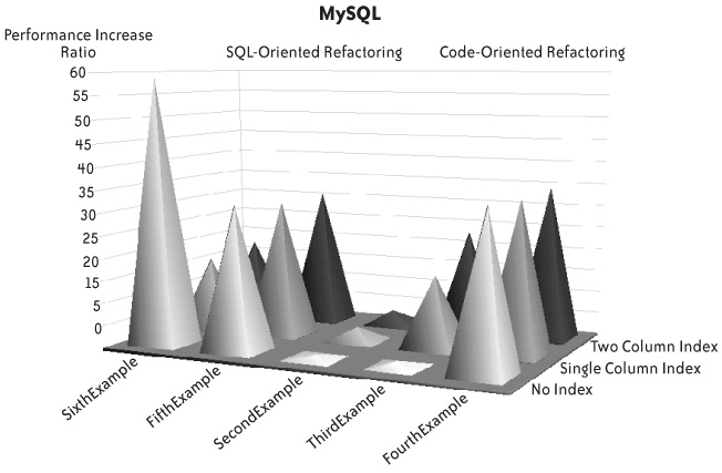
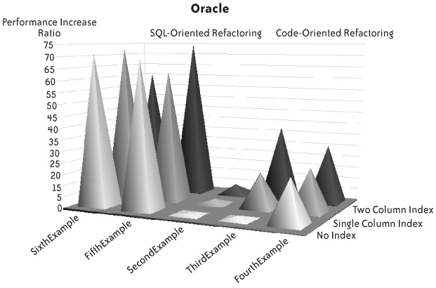
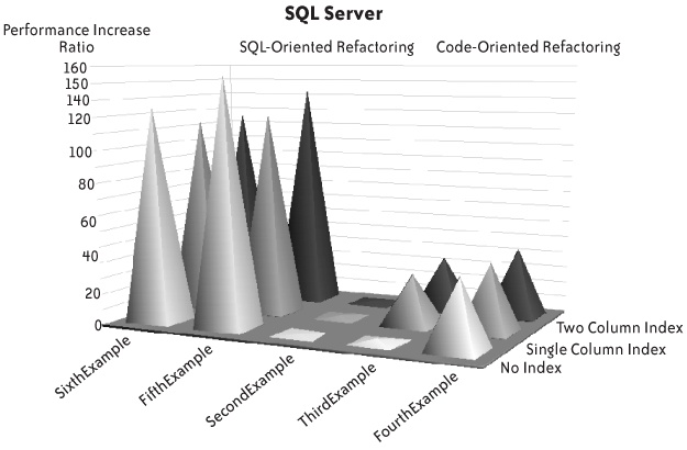
I plotted the following:
- On one axis
The version of the program that has the minimally improved code in the middle (SecondExample.java). On one side we have code-oriented refactoring: ThirdExample.java, which minimizes the calls in lookup functions, and FourthExample.java, which is identical except for a query with a subquery replacing two queries. On the other side we have SQL-oriented refactoring, in which the lookup functions have vanished, but with two variants of the main SQL statement.
- On the other axis
The different additional indexes (no index, single-column index, and two-column index).
Two characteristics are immediately striking:
The similarity of performance improvement patterns, particularly in the case of Oracle and SQL Server.
The fact that the âindexing-onlyâ approach, which is represented in the figures by SecondExample with a single-column index or a two-column index, leads to a performance improvement that varies between nonexistent and extremely shy. The true gains are obtained elsewhere, although with MySQL there is an interesting case when the presence of an index severely cripples performance (compared to what it ought to be), as you can see with SixthExample.
The best result by far with MySQL is obtained, as with all other products, with a single query and no additional index. However, it must be noted not only that in this version the optimizer may sometimes try to use indexes even when they are harmful, but also that it is quite sensitive to the way queries are written. The comparison between FifthExample and SixthExample denotes a preference for joins over (logically equivalent) subqueries.
By contrast, Oracle and SQL Server appear in this example like the tweedledum and tweedledee of the database world. Both demonstrate that their optimizer is fairly insensitive to syntactical variations (even if SQL Server denotes, contrary to MySQL, a slight preference for subqueries over joins), and is smart enough in this case to not use indexes when they donât speed up the query (the optimizers may unfortunately behave less ideally when statements are much more complicated than in this simple example, which is why Iâll devote Chapter 5 to statement refactoring). Both Oracle and SQL Server are the reliable workhorses of the corporate world, where many IT processes consist of batch processes and massive table scans. When you consider the performance of Oracle with the initial query, three minutes is a very decent time to perform several hundred full scans of a two-million-row table (on a modest machine). But you mustnât forget that a little reworking brought down the time required to perform the same process (as in âbusiness requirementâ) to a little less than two seconds. Sometimes superior performance when performing full scans just means that response times will be mediocre but not terrible, and that serious code defects will go undetected. Only one full scan of the transaction table is required by this process. Perhaps nothing would have raised an alarm if the program had performed 10 full scans instead of 252, but it wouldnât have been any less faulty.
As I have pointed out, the two different approaches I took to refactoring my sample code are incompatible: in one case, I concentrated my efforts on improving functions that the other case eliminated. It seems pretty evident from Figures Figure 1-1, Figure 1-2, and Figure 1-3 that the best approach with all products is the "single queryâ approach, which makes creating a new index unnecessary. The fact that any additional index is unnecessary makes sense when you consider that one areaid value defines a perimeter that represents a significant subset in the table. Fetching many rows with an index is costlier than scanning them (more on this topic in the next chapter). An index is necessary only when we have one query to return accountid values and one query to get transaction data, because the date range is selective for one accountid valueâbut not for the whole set of accounts. Using indexes (including the creation of appropriate additional indexes), which is often associated in peopleâs minds with the traditional approach to SQL tuning, may become less important when you take a refactoring approach.
I certainly am not stating that indexes are unimportant; they are highly important, particularly in online transaction processing (OLTP) environments. But contrary to popular belief, they are not all-important; they are just one factor among several others, and in many cases they are not the most important element to consider when you are trying to deliver better performance.
Most significantly, adding a new index risks wreaking havoc elsewhere. Besides additional storage requirements, which can be quite high sometimes, an index adds overhead to all insertions into and deletions from the table, as well as to updates to the indexed columns; all indexes have to be maintained alongside the table. It may be a minor concern if the big issue is the performance of queries, and if we have plenty of time for data loads.
There is, however, an even more worrying fact. Just consider, in Figure 1-1, the effect of the index on the performance of SixthExample.java: it turned a very fast query into a comparatively slow one. What if we already have queries written on the same pattern as the query in SixthExample.java? I may fix one issue but create problem queries where there were none. Indexing is very important, and Iâll discuss the matter in the next chapter, but when something is already in production, touching indexes is always a risk. [4] The same is true of every change that affects the database globally, particularly parameter changes that impact even more queries than an index.
There may be other considerations to take into account, though. Depending on the development teamâs strengths and weaknesses, to say nothing of the skittishness of management, optimizing lookup functions and adding an index may be perceived as a lesser risk than rethinking the processâs core query. The preceding example is a simple one, and the core query, without being absolutely trivial, is of very moderate complexity. There may be cases in which writing a satisfactory query may either exceed the skills of developers on the team, or be impossible because of a bad database design that cannot be changed.
In spite of the lesser performance improvement and the thorough nonregression tests required by such a change to the database structure as an additional index, separately improving functions and the main query may sometimes be a more palatable solution to your boss than what I might call grand refactoring. After all, adequate indexing brought performance improvement factors of 16 to 35 with ThirdExample.java, which isnât negligible.
It is sometimes wise to stick to âacceptableâ even when âexcellentâ is within reachâyou can always mention the excellent solution as the last option.
Whichever solution you finally settle for, and whatever the reason, you must understand that the same idea drives both refactoring approaches: minimizing the number of calls to the database server, and in particular, decreasing the shockingly high number of queries issued by the AboveThreshold() function that we got in the initial version of the code.
The greatest difficulty when undertaking a refactoring assignment is, without a shadow of a doubt, assessing how much improvement is within your grasp.
When you consider the alternative option of âthrowing more hardware to the performance problem,â you swim in an ocean of figures: number of processors, CPU frequency, memory, disk transfer ratesâ¦and of course, hardware price. Never mind the fact that more hardware sometimes means a ridiculous improvement and, in some cases, worse performance [5] (this is when a whole range of improvement possibilities can be welcome).
It is a deeply ingrained belief in the subconscious minds of chief information officers (CIOs) that twice the computing power will mean better performanceâif not twice as fast, at least pretty close. If you confront the hardware option by suggesting refactoring, you are fighting an uphill battle and you must come out with figures that are at least as plausible as the ones pinned on hardware, and are hopefully truer. As Mark Twain once famously remarked to a visiting fellow journalist [6]:
Get your facts first, and then you can distort âem as much as you please.
Using a system of trial and error for an undefined number of days, trying random changes and hoping to hit the nail on the head, is neither efficient nor guarantees success. If, after assessing what needs to be done, you cannot offer credible figures for the time required to implement the changes and the expected benefits, you simply stand no chance of proving yourself right unless the hardware vendor is temporarily out of stock.
Assessing by how much you can improve a given program is a very difficult exercise. First, you must define in which unit you are going to express âhow much.â Needless to say, what users (or CIOs) would probably love to hear is âwe can reduce the time this process needs by 50%â or something similar. But reasoning in terms of response time is very dangerous and leads you down the road to failure. When you consider the hardware option, what you take into account is additional computing power. If you want to compete on a level field with more powerful hardware, the safest strategy is to try to estimate how much power you can spare by processing data more efficiently, and how much time you can save by eliminating some processes, such as repeating thousands or millions of times queries that need to run just once. The key point, therefore, is not to boast about a hypothetical performance gain that is very difficult to predict, but to prove that first there are some gross inefficiencies in the current code, and second that these inefficiencies are easy to remedy.
The best way to prove that a refactoring exercise will pay off is probably to delve a little deeper into the trace file obtained with Oracle for the initial program (needless to say, analysis of SQL Server runtime statistics would give a similar result).
The Oracle trace file gives detailed figures about the CPU and elapsed times used by the various phases (parsing, execution, and, for select statements, data fetching) of each statement execution, as well as the various âwait eventsâ and time spent by the DBMS engine waiting for the availability of a resource. I plotted the numbers in Figure 1-4 to show how Oracle spent its time executing the SQL statements in the initial version of this chapterâs example.
You can see that the 128 seconds the trace file recorded can roughly be divided into three parts:
CPU time consumed by Oracle to process the queries, which you can subdivide into time required by the parsing of statements, time required by the execution of statements, and time required for fetching rows. Parsing refers to the analysis of statements and the choice of an execution path. Execution is the time required to locate the first row in the result set for a
selectstatement (it may include the time needed to sort this result set prior to identifying the first row), and actual table modification for statements that change the data. You might also see recursive statements, which are statements against the data dictionary that result from the program statements, either during the parsing phase or, for instance, to handle space allocation when inserting data. Thanks to my using prepared statements and the absence of any massive sort, the bulk of this section is occupied by the fetching of rows. With hardcoded statements, each statement appears as a brand-new query to the SQL engine, which means getting information from the data dictionary for analysis and identification of the best execution plan; likewise, sorts usually require dynamic allocation of temporary storage, which also means recording allocation data to the data dictionary.Wait time, during which the DBMS engine is either idle (such as
SQL*Net message from client, which is the time when Oracle is merely waiting for an SQL statement to process), or waiting for a resource or the completion of an operation, such as I/O operations denoted by the twodb fileevents (db file sequential readprimarily refers to index accesses, anddb file scattered readto table scans, which is hard to guess when one doesnât know Oracle), both of which are totally absent here. (All the data was loaded in memory by prior statistical computations on tables and indexes.) Actually, the only I/O operation we see is the writing to logfiles, owing to the auto-commit mode of JDBC. You now understand why switching auto-commit off changed very little in that case, because it accounted for only 1% of the database time.Unaccounted time, which results from various systemic errors such as the fact that precision cannot be better than clock frequency, rounding errors, uninstrumented Oracle operations, and so on.
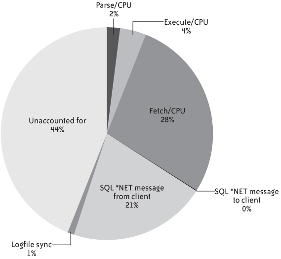
If I had based my analysis on the percentages in Figure 1-4 to try to predict by how much the process could be improved, I would have been unable to come out with any reliable improvement ratio. This is a case when you can be tempted to follow Samuel Goldwynâs advice:
Never make forecasts, especially about the future.
For one thing, most waits are waits for work (although the fact that the DBMS is waiting for work should immediately ring a bell with an experienced practitioner). I/O operations are not a problem, in spite of the missing index. You could expect an index to speed up fetch time, but the previous experiments proved that index-induced improvement was far from massive. If you naively assume that it would be possible to get rid of all waits, including time that is unaccounted for, you would no less naively assume that the best you can achieve is to divide the runtime by about 3âor 4 with a little bit of luckâwhen by energetic refactoring I divided it by 100. It is certainly better to predict 3 and achieve 100 than the reverse, but it still doesnât sound like you know what you are doing.
How I obtained a factor of 100 is easy to explain (after the deed is done): I no longer fetched the rows, and by reducing the process to basically a single statement I also removed the waits for input from the application (in the guise of multiple SQL statements to execute). But waits by themselves gave me no useful information about where to strike; the best I can get from trace files and wait analysis is the assurance that some of the most popular recipes for tuning a database will have no or very little effect.
Wait times are really useful when your changes are narrowly circumscribed, which is what happens when you tune a system: they tell you where time is wasted and where you should try to increase throughput, by whatever means are at your disposal. Somehow wait times also fix an upper bound on the improvement you can expect. They can still be useful when you want to refactor the code, as an indicator of the weaknesses of the current version (although there are several ways to spot weaknesses). Unfortunately, they will be of little use when trying to forecast performance after code overhaul. Waiting for input for the application and much-unaccounted-for time (when the sum of rounding errors is big, it means you have many basic operations) are both symptoms of a very âchattyâ application. However, to understand why the application is so chatty and to ascertain whether it can be made less chatty and more efficient (other than by tuning low-level TCP parameters) I need to know not what the DBMS is waiting for, but what keeps it busy. In determining what keeps a DBMS busy, you usually find a lot of operations that, when you think hard about them, can be dispensed with, rather than done faster. As Abraham Maslow put it:
What is not worth doing is not worth doing well.
Tuning is about trying to do the same thing faster; refactoring is about achieving the same result faster. If you compare what the database is doing to what it should or could be doing, you can issue some reliable and credible figures, wrapped in suitable oratorical precautions. As I have pointed out, what was really interesting in the Oracle trace wasnât the full scan of the two-million-row table. If I analyze the same trace file in a different way, I can create Table 1-7. (Note that the elapsed time is smaller than the CPU time for the third and fourth statements; it isnât a typo, but what the trace file indicatesâjust the result of rounding errors.)
Table 1-7. What the Oracle trace file says the DBMS was doing
When looking at Table 1-7, you may have noticed the following:
The first striking feature in Table 1-7 is that the number of rows returned by one statement is most often the number of executions of the next statement: an obvious sign that we are just feeding the result of one query into the next query instead of performing joins.
The second striking feature is that all the elapsed time, on the DBMS side, is CPU time. The two-million-row table is mostly cached in memory, and scanned in memory. A full table scan doesnât necessarily mean I/O operations.
We query the
thresholdstable more than 30,000 times, returning one row in most cases. This table contains 20 rows. It means that each single value is fetched 1,500 times on average.Oracle gives an elapsed time of about 43 seconds. The measured elapsed time for this run was 128 seconds. Because there are no I/O operations worth talking about, the difference can come only from the Java code runtime and from the âdialogueâ between the Java program and the DBMS server. If we decrease the number of executions, we can expect the time spent waiting for the DBMS to return from our JDBC calls to decrease in proportion.
We are already getting a fairly good idea of what is going wrong: we are spending a lot of time fetching data from transactions, we are querying thresholds of 1,500 more times than needed, and we are not using joins, thus multiplying exchanges between the application and the server.
But the question is, what can we hope for? Itâs quite obvious from the figures that if we fetch only 20 times (or even 100 times) from the thresholds table, the time globally taken by the query will dwindle to next to nothing. More difficult to estimate is the amount of time we need to spend querying the transactions table, and we can do that by imagining the worst case. There is no need to return a single transaction several times; therefore, the worst case I can imagine is to fully scan the table and return about one sixty-fourth (2,000,000 divided by 31,000) of its rows. I can easily write a query that, thanks to the Oracle pseudocolumn that numbers rows as they are returned (I could have used a session variable with another DBMS), returns one row every 65 rows, and run this query under SQL*Plus as follows:
SQL> set timing on
SQL> set autotrace traceonly
SQL> select *
  2  from (select rownum rn, t.*
  3        from transactions t)
  4  where mod(rn, 65) = 0
  5  /

30769 rows selected.

Elapsed: 00:00:03.67

Execution Plan
----------------------------------------------------------
Plan hash value: 3537505522

--------------------------------------------------------------------------------
| Id | Operation           | Name       | Rows |  Bytes| Cost (%CPU)| Time     |
--------------------------------------------------------------------------------
|  0 | SELECT STATEMENT    |            | 2000K|   125M| 2495    (2)| 00:00:30 |
|* 1 |  VIEW               |            | 2000K|   125M| 2495    (2)| 00:00:30 |
|  2 |   COUNT             |            |      |       |            |          |
|  3 |    TABLE ACCESS FULL|TRANSACTIONS| 2000K|    47M| 2495    (2)| 00:00:30 |
------------------------------------------------------------------------------

Predicate Information (identified by operation id):
---------------------------------------------------

   1 - filter(MOD("RN",65)=0)

Statistics
----------------------------------------------------------
          1  recursive calls
          0  db block gets
      10622  consistent gets
       8572  physical reads
          0  redo size
    1246889  bytes sent via SQL*Net to client
      22980  bytes received via SQL*Net from client
       2053  SQL*Net roundtrips to/from client
          0  sorts (memory)
          0  sorts (disk)
      30769  rows processed
I have my full scan and about the same number of rows returned as in my programâand it took less than four seconds, in spite of not having found data in memory 8 times out of 10 (the ratio of physical reads to consistent gets + db block gets that is the count of logical references to the Oracle blocks that contain data). This simple test is the proof that there is no need to spend almost 40 seconds fetching information from transactions.
Short of rewriting the initial program, there isnât much more that we can do at this stage. But we have a good proof of concept that is convincing enough to demonstrate that properly rewriting the program could make it use less than 5 seconds of CPU time instead of 40; I emphasize CPU time here, not elapsed time, because elapsed time includes wait times that I know will vanish but on which I cannot honestly pin any figure. By talking CPU time, I can compare the result of code rewriting to buying a machine eight times faster than the current one, which has a price. From here you can estimate how much time it will take to refactor the program, how much time will be required for testing, whether you need external help in the guise of consultingâall things that depend on your environment, the amount of code that has to be revised, and the strengths of the development team. Compute how much it will cost you, and compare this to the cost of a server that is eight times more powerful (as in this example) than your current server, if such a beast exists. You are likely to find yourself in a very convincing positionâand then it will be your mission to deliver and meet (or exceed) expectations.
Assessing whether you can pin any hope on refactoring, therefore, demands two steps:
Find out what the database is doing. Only when you know what your server is doing can you notice the queries that take the whole edifice down. Itâs then that you discover that several costly operations can be grouped and performed as a single pass, and that therefore, this particular query has no reason to be executed as many times as it is executed, or that a loop over the result of a query to execute another query could be replaced by a more efficient join.
Analyze current activity with a critical eye, and create simple, reasonable proofs of concept that demonstrate convincingly that the code could be much more efficient.
Most of this book is devoted to describing patterns that are likely to be a fertile ground for refactoring and, as a consequence, to give you ideas about what the proof of concept might be. But before we discuss those patterns, letâs review how you can identify SQL statements that are executed.
You have different ways to monitor SQL activity on your database. Every option isnât available with every DBMS, and some methods are more appropriate for test databases than for production databases. Furthermore, some methods allow you to monitor everything that is happening, whereas others let you focus on particular sessions. All of them have their use.
Oracle started with version 6 what is now a popular trend: dynamic views, relational (tabular) representations of memory structures that the system updates in real time and that you can query using SQL. Some views, such as v$session with Oracle, sys.dm_exec_requests with SQL Server, and information_schema.processlist with MySQL, let you view what is currently executing (or has just been executed). However, sampling these views will not yield anything conclusive unless you also know either the rate at which queries are executed or their duration. The dynamic views that are truly interesting are those that map the statement cache, complete with counters regarding the number of executions of each statement, the CPU time used by each statement, the number of basic data units (called blocks with Oracle and pages elsewhere) referenced by the statement, and so on. The number of data pages accessed to execute the query is usually called the logical read and is a good indicator of the amount of work required by a statement. The relevant dynamic views are v$sqlstats [7] with Oracle and sys.dm_exec_query_stats with SQL Server. As you can infer from their names, these views cannot be queried by every Tom, Dick, or Harry, and you may need to charm your DBA to get the license to drill. They are also the basis for built-in (but sometimes separately licensed) monitoring utilities such as Oracleâs Automatic Workload Repository (AWR) and companion products.
Dynamic views are a wonderful source of information, but they have three issues:
They give instant snapshots, even if the counters are cumulative. If you want to have a clear picture of what happens during the day, or simply for a few hours, you must take regular snapshots and store them somewhere. Otherwise, you risk focusing on a big costly query that took place at 2 a.m. when no one cared, and you may miss the real issues. Taking regular snapshots is what Oracleâs Statspack utility does, as well as Oracleâs ASH (which stands for Active Session History) product, which is subject to particular licensing conditions (in plain English, you have to pay a lot more if you want it).
Querying memory structures that display vital and highly volatile information takes time that may be modest compared to many of the queries on the database, but may harm the whole system. This is not equally true of all dynamic views (some are more sensitive than others), but to return consistent information, the process that returns data from the innermost parts of the DBMS must somehow lock the structures while it reads them: in other words, while you read the information stating that one particular statement has been executed 1,768,934 times, the process that has just executed it again and wants to record the deed must wait to update the counter. It will not take long, but on a system with a very big cache and many statements, it is likely that your
selecton the view, which, behind the scenes, is a traversal of some complicated memory structure, will hamper more than one process. You mustnât forget that youâll have to store what is returned to record the snapshot, necessarily slowing down your query. In other words, you donât want to poll dynamic views at a frantic rate, because if you do, hardly anybody else will be able to work properly.As a result, there is a definite risk of missing something. The problem is that counters are associated with a cached statement. Whatever way you look at the problem, the cache has a finite size, and if you execute a very high number of different statements, at some point the DBMS will have to reuse the cache that was previously holding an aged-out statement. If you execute a very, very big number of different statements, rotation can be quick, and pop goes the SQL, taking counters with it. Itâs easy to execute a lot of different statements; you just have to hardcode everything and shun prepared statements and stored procedures.
Acknowledging the last two issues, some third-party tool suppliers provide programs that attach to the DBMS memory structures and read them directly, without incurring the overhead of the SQL layer. This allows them to scan memory at a much higher rate with a minimized impact over regular DBMS activity. Their ability to scan memory several times per second may make particularly surprising the fact that, for instance, many successful Oracle DBAs routinely take snapshots of activity at intervals of 30 minutes.
Actually, missing a statement isnât something that is, in itself, very important when you try to assess what the database server is busy doing. You just need to catch important statements, statements that massively contribute to the load of the machine and/or to unsatisfactory response times. If I grossly simplify, I can say that there are two big categories of statements worth tuning:
The big, ugly, and slow SQL statements that everyone wants to tune (and that are hard to miss)
Statements which are not, by themselves, costly, but which are executed so many times that the cumulative effect is very costly
In the sample program at the beginning of this chapter, we encountered examples of both categories: the full scan on a two-million-row table, which can qualify as a slow query, and the super-fast, frequently used lookup functions.
If we check the contents of the statement cache at regular intervals, we will miss statements that were first executed and that aged out of the cache between two inspections. I have never met an application that was executing an enormous quantity of different statement patterns. But the worry is that a DBMS will recognize two statements to be identical only when the text is identical, byte for byte:
If statements are prepared and use variables, or if we call stored procedures, even if we poll at a low rate, we will get a picture that may not be absolutely complete but which is a fair representation of what is going on, because statements will be executed over and over again and will stay in the cache.
If, instead of using prepared statements, you build them dynamically, concatenating constant values that are never the same, then your statements may be identical in practice, but the SQL engine will only see and report myriad different statementsâall very fast, all executed onceâwhich will move in and out of the cache at lightning speed to make room for other similar statements. If you casually check the cache contents, you will catch only a small fraction of what really was executed, and you will get an inaccurate idea of what is going on, because the few statements that may correctly use parameters will take a disproportionate âweightâ compared to the hardcoded statements that may be (and probably are) the real problem. In the case of SQL Server, for which stored procedures get preferential treatment as far as cache residency is concerned, SQL statements executed outside stored procedures, because they are more volatile, may look less harmful than they really are.
To picture exactly how this might work in practice, suppose we have a query (or stored procedure) that uses parameters and has a cost of 200 units, and a short, hardcoded query that has a cost of 3 units. Figure that, between 2 times when we query the statement cache, the costlier query is executed 5 times and the short query 4,000 timesâlooking like 4,000 distinct statements. Furthermore, letâs say that our statement cache can hold only 100 queries (something much lower than typical real values). If you check the top five queries, the costlier query will appear with a cumulated cost of 1,000 (5 x 200), and will be followed by four queries with a comparatively ridiculous cost of 3 (1 x 3 each time). Moreover, if you try to express the relative importance of each query by comparing the cost of each to the cumulated cost of cached statements, you may wrongly compute the full value for the cache as 1 x 1,000 + 99 x 3 = 1,297 (based on current cache values), of which the costly query represents 77%. Using the current cache values alone grossly underreports the total cost of the fast query. Applying the cost units from the current cache to the total number of statements executed during this period, the actual full cost for the period was 5 x 200 + 4,000 x 3 = 13,000, which means that the âcostlyâ query represents only 7% of the real costâand the âfastâ query 93%.
You must therefore collect not only statements, but also global figures that will tell you which proportion of the real load is explained by the statements you have collected. Therefore, if you choose to query v$sqlstats with Oracle (or sys.dm_exec_query_stats with SQL Server), you must also find global counters. With Oracle, you can find them easily within v$sysstat: youâll find there the total number of statements that were executed, the CPU time that has been consumed, the number of logical reads, and the number of physical I/O operations since database startup. With SQL Server, you will find many key figures as variables, such as @@CPU_BUSY, @@TIMETICKS, @@TOTAL_READ, and @@TOTAL_WRITE. However, the figure that probably represents the best measure of work performed by any DBMS is the number of logical reads, and it is available from sys.dm_os_performance_counters as the value associated with the rather misleadingly named counter, Page lookups/sec (itâs a cumulative value and not a rate).
Now, what do you do if you realize that by probing the statement cache, say, every 10 minutes, you miss a lot of statements? For instance, with my previous example, I would explain a cost of 1,297 out of 13,000. This is, in itself, a rather bad sign, and as weâll see in the next chapter, there are probably significant gains to expect from merely using prepared statements. A solution might be to increase the frequency that is used for polling, but as I explained, probing may be costly. Polling too often can deliver a fatal blow to a system that is already likely to be in rather bad health.
When you are missing a lot of statements, there are two solutions for getting a less distorted view of what the database is doing: one is to switch to logfile-based analysis (my next topic), and the other is to base analysis on execution plans instead of statement texts.
The slot in the statement cache associated with each statement also contains a reference to the execution plan associated with that statement (plan_hash_value in Oracleâs v$sqlstats, plan_handle in SQL Serverâs sys.dm_exec_query_stats; note that in Oracle, each plan points to the address of a âparent cursorâ instead of having statements pointing to a plan, as with SQL Server). Associated plan statistics can respectively be found in v$sql_plan_statistics (which is extremely detailed and, when statistics collection is set at a high level for the database, provides almost as much information as trace files) and sys.dm_exec_cached_plans.
Execution plans are not what we are interested in; after all, if we run FirstExample.java with an additional index, we get very nice execution plans but still pathetic performance. However, hardcoded statements that differ only in terms of constant values will, for the most part, use the same execution plan. Therefore, aggregating statement statistics by the associated execution plan instead of doing it by text alone will give a much truer vision of what the database is really doing. Needless to say, execution plans are not a perfect indicator. Some changes at the session level can lead to different execution plans with the same statement text for two sessions (we can also have synonyms resolving to totally different objects); and, any simple query on an unindexed table will result in the same table scan, whichever column(s) you use for filtering rows. But even if there isnât a one-to-one correspondence between a statement pattern and an execution plan, execution plans (with an associated sample query) will definitely give you a much better idea of what type of statement really matters than statement text alone when numbers donât add up with statements.
It is possible to make all DBMS products log SQL statements that are executed. Logging is based on intercepting the statement before (or after) it is executed and writing it to a file. Interception can take place in several locations: where the statement is executed (on the database server), or where it is issued (on the application side)âor somewhere in between.
Server-side logging. Server-side logging is the type of logging most people think of. The scope can be either the whole system or the current session. For instance, when you log slow queries with MySQL by starting the server with the --log-slow-queries option, it affects every session. The snag is that if you want to collect interesting information, the amount of data you need to log is often rather high. For instance, if we run FirstExample.java against a MySQL server that was started with --log-slow-queries, we find nothing in the logfile when we have the additional index on transactions: there is no slow query (itâs the whole process that is slow), and I have made the point that it can nevertheless be made 15 to 20 times faster. Logging these slow queries can be useful to administrators for identifying big mistakes and horrid queries that have managed to slip into production, but it will tell you nothing about what the database is truly doing as long as each unit of work is fast enough.
If you really want to see what matters, therefore, you must log every statement the DBMS executes (by starting the MySQL server with --log, setting the global general_log variable to ON, and by setting the Oracle sql_trace parameter to true or activating event 10046; if you are using SQL Server, call sp_trace_create to define your trace file, then sp_trace_setevent multiple times to define what you want to trace, and then sp_trace_setstatus to start tracing). In practice, this means you will get gigantic logfiles if you want to put a busy server in trace mode. (Sometimes you will get many gigantic logfiles. Oracle will create one trace file per server process, and it isnât unusual to have hundreds of them. For SQL Server, it may create a new trace file each time the current file becomes too big.) This is something you will definitely want to avoid on a production server, particularly if it is already showing some signs of running out of breath. In addition to the overhead incurred by timing, catching, and writing statements, you incur the risk of filling up disks, a situation that a DBMS often finds uncomfortable. However, it may be the smart thing to do within a good-quality assurance environment and if you are able to generate a load that simulates production.
When you want to collect data on a production system, though, it is usually safer to trace a single session, which you will do with MySQL by setting the sql_log_off session variable to ON and with Oracle by executing:
alter session set timed_statistics=true,
alter session set max_dump_file_size=unlimited;
alter session se tracefile_identifier='something meaningful';
alter session set events '10046 trace name context forever, level 8';
The level parameter for the event specifies how much information to collect. Possible values are:
1 (displays basic trace information)
4 (displays bind variables, values that are passed)
8 (displays wait statistics)
12 (displays wait statistics and bind variables)
With SQL Server, you need to call sp_trace_filter to specify the Service Profile Identifier (SPID) or login name (depending on which is more convenient) that you want to trace before turning tracing on.
Because it isnât always convenient to modify an existing program to add this type of statement, you can ask a DBA either to trace your session when it is started (DBAs sometimes can do that) or, better perhaps, to create a special user account on which a login trigger turns tracing on whenever you connect to the database through this account.
Client-side logging. Unfortunately, there are some downsides to server-side logging:
Because logging takes place on the server, it consumes resources that may be in short supply and that may impact global performance even when you are tracing a single session.
Tracing a single session may prove difficult when you are using an application server that pools database connections: there is no longer a one-to-one link between the end-user session and a database session. As a result, you may trace more or less than you initially intended and find it difficult to get a clear picture of activity out of trace files without the proper tools.
When you are a developer, the production database server is often off-limits. Trace files will be created under accounts you have no access to, and you will depend on administrators to obtain and process the trace files you generate. Depending on people who are often extremely busy may not be very convenient, particularly if you want to repeat tracing operations a number of times.
An alternative possibility is to trace SQL statements where they are issued: on the application server side. The ideal case is, of course, when the application itself is properly instrumented. But there may be other possibilities:
If you are using an application server such as JBoss, WebLogic, or WebSphereâor simple JDBCâyou can use the free p6spy tracer, which will time each statement that is executed.
With JDBC, you can sometimes enable logging in the JDBC driver. (For instance, you can do this with the MySQL JDBC driver.)
In-between logging. Also available are hybrid solutions. An example is SQL Serverâs SQL Profiler, which activates server-side traces but is a client tool that receives trace data from the server. Although SQL Profiler is much more pleasant to use than the T-SQL system procedures, the data traffic that flows toward the tool somewhat counterbalances the creation of a trace file on the server, and it is often frowned upon as not being as efficient as âpureâ server-side logging.
I must mention that you can trap and time SQL statements in other ways, even if they require a fair amount of programming; you may encounter these techniques in some third-party products. When you âtalkâ to a DBMS you actually send your SQL statements to a TCP/IP port on the server. It is sometimes possible to have a program that listens on a port other than the port on which the true DBMS listener program is listening; that program will trap and log whatever you send it before forwarding it to the DBMS. Sometimes the DBMS vendor officially acknowledges this method and provides a true proxy (such as MySQL Proxy, or the pioneering Sybase Open Server). The technique of using a proxy is similar to the implementation of web filtering through a proxy server.
With trace files, you will not miss any statements, which means you may get a lot of data. I already explained that if statements are hardcoded, you will miss many of them, and you will, generally speaking, get a biased view of what is going on if you poll the statement cache. With trace files, the problem is slightly different: you will get so many statements in your file that it may well be unusable, even after processing raw logfiles with a tool such as tkprof for Oracle or mysqlsla [8] for MySQL.
One good way to handle data afterward is to load it into a database and query it! Oracleâs tkprof has long been able to generate insert statements instead of a text report, and SQL Serverâs tools and the fn_trace_gettable() function make loading a trace file into a table a very easy operation. There is only one snag: you need a database to load into. If you have no development database at your disposal, or if you are a consultant who is eager to keep your work separate from your customers', think of SQLite: [9] you can use it to create a file in which data is stored in tables and queried with SQL, even if loading the trace file may require a little coding.
The problem is that even with a database at your disposal, the volume of data to analyze may be daunting. I once traced with Oracle (knowing that querying v$sqlstats would give me nothing because most statements were hardcoded) a program, supplied by a third-party editor, that was taking around 80 minutes to generate a 70-page report. That was on a corporate-grade Sun server running Solaris; the text report resulting from the output of tkprof was so big that I couldnât open it with vi and carried out my analysis using commands such as grep, sed, awk, and wc (if you are not conversant in Unix-based operating systems, these are powerful but rather low-level command-line utilities). The purpose wasnât to refactor the code (there was no source code to modify, only binary programs were available), but to audit the client/server application and understand why it was taking so long to run on a powerful server while the same report, with the same data, was taking much less time on the laptop of the vendorâs technical consultant (who was all the same advising to buy a more powerful server). The trace file nevertheless gave me the answer: there were 600,000 statements in the file; average execution time was 80 minutes / 600,000 = 8 milliseconds. Oracle was idle 90% of the time, actually, and most of the elapsed time was local area network (LAN) latency. I would have loved to have been given the opportunity to refactor this program. It would have been easy to slash execution time by several orders of magnitude.
You must process trace files (or trace data) if you want to get anything out of them. If statements are hardcoded, itâs better to be a regular expression fiend and replace all constant strings with something fixed (say, 'constant') and all number constants with something such as 0. This will be your only chance to be able to aggregate statements that are identical from the standpoint of the application but not from that of the DBMS. You may have to massage the trace file so as to assign one timestamp to every line (the only way to know exactly when each statement was executed). After thatâs done, you must aggregate any timing information you have and count how many identical patterns you have. You will then get solid material that you analyze to see what you can do to improve performance.
Letâs now see how we can analyze data we have collected either through cache probing or through logging and what it tells us about performance improvement possibilities.
In all the cases I have experienced, most of the database load for considerable parts of the day (or night) was the result of fewer than 10 queries or query patterns, and you can usually narrow the âqueries that countâ down to 4 or 5.
Most of these queries will be very big queries, or fast queries that are executed too often. As we saw previously, even if we cannot ignore big queries, focusing on single queries may make us miss big performance gains. We must step back and relate SQL activity to business activity and check whether what is done often can be done less frequently or not at all. If we succeed in identifying queries that we could run less often, we must determine how much CPU time they currently use and compute how much we can save. This is easier and safer to do than trying to predict response times. When you buy a more powerful server, all you really know is that you are in fact buying CPU time, and the vendorâs own benchmark lets you know the power ratio between your current server and the projected one. If you can plausibly demonstrate that refactoring the code would decrease CPU consumption by 20% at peak time, for all practical purposes that means the proposed refactoring effort would have the same result as buying a new server that is 20% more powerful, minus migration costs.
Actually, there is more to refactoring than the reduction of CPU consumption on the server, and I hope that Figure 1-5 will give you a good understanding of the real benefits to expect. In many poorly written applications, you have an incessant chat between the application side and the server side. Suppose we have a cursor loopâsome select statement that returns a number of rows and performs, say, an update in the loop. The application will issue a number of database calls:
First it will issue an
executecall that will analyze theselectstatement, parse it, determine an execution plan if necessary, and do whatever is required (including sorts) to locate the first row to return.Then it will iterate on
fetchcalls that will return rows, either one by one or, sometimes, in batches.While still in the loop, another
executecall will perform anupdate. Because this operation changes the database, no other call follows theexecutefor this statement.
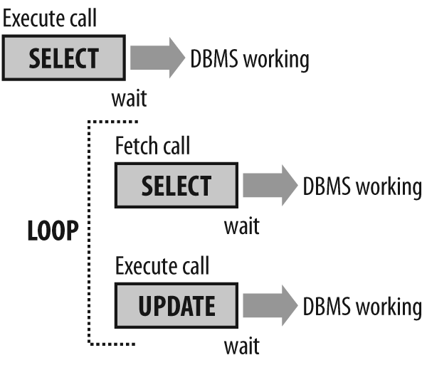
Basic database calls are synchronous, which means that most applications are suspended and they wait until the DBMS is done with its side of the job. This wait time is actually the assembly of several components:
The communication time it takes for your statement to reach the server
The time it takes the server to compute a checksum on your statement and check whether it already has a matching execution plan in its cache
Optionally, the time it takes to actually parse the statement and determine an execution plan
The actual execution time for your statement, a âservice timeâ that includes CPU time and, possibly, I/O wait time or wait time for a resource that cannot be shared
The time it takes to receive data from the server or obtain execution information such as a return code and the number of rows processed
By tuning statements on a unitary basis, you improve only the fourth component. If we manage to get rid of unnecessary calls, as we did in the earlier example by improving lookup functions, we can remove in a loop the execution of the five components a significant number of times. If we get rid of the loop, we get rid of all the overhead at once.
Now that we know the top statements that keep our DBMS busy, we should look for the following several patterns:
If the statements that are (globally) the most costly are fast statements that are executed a large number of times, you stand a high chance of success with refactoring, and giving an estimate is reasonably easy. If you have a static table, such as a reference lookup table, for which the average number of queries per active session is greater than the number of rows in the table, on average each row is called several times. Very often, âseveralâ doesnât mean two or three times, but thousands of times or more. You can be sure that you can reduce this number of calls and therefore spare the CPU consumption attached with each execution. You usually find this type of call when you are performing transcoding, currency conversion, or calendar computations, among other operations. I will discuss in more detail how to minimize the number of calls in Chapter 3.
If you have some very costly statements, predicting how much you can save by rewriting statements in a better way is much more difficult; if the indexing strategy, which Iâll discuss in Chapter 2, is sound, and if, as youâll see in Chapter 3, there is no complicated view that can be simplified, your success here strongly depends on your SQL skills. I hope that after you read Chapter 5 your chances of significantly improving a badly written statement will be in the 40% to 60% range.
When you see several similar updates applied to the same tables, and if your SQL skills are not too rusty, you also stand a very good chance of merging some of them, as Iâll discuss in Chapter 6. Doing in one statement what two statements were previously doing routinely improves (surprise!) performance by a factor of two; unfortunately, sometimes you canât do this. A relatively safe assumption is to bet on a possible improvement in 20% to 25% of cases.
When you can describe which statements load the server and can assign to each of them a probability of improving them in terms of CPU consumption, youâll have figures that you can compare to faster hardware, but never talk response times. CPU time is just one component of response time, and you can improve response times a lot by getting rid of all the time wasted in communication between the application and the DBMS. Now, the difficulty for you will be to estimate at what cost you can obtain these gains. The following chapters will help you to refine estimates of what you can get, and at what price.
[2] MySQL 5.1.
[3] SQL Server 2005 and Oracle 11.
[4] Even if, in the worst case, dropping an index (or making it invisible with Oracle 11 and later) is an operation that can be performed relatively quickly.
[5] Through aggrieved contention. It isnât as frequent as pathetic improvement, but it happens.
[6] No less than Rudyard Kipling, who told of his interview of Twain in From Sea to Sea.
[7] Available since Oracle 10, but the information was available in v$sql in previous versions.
Get Refactoring SQL Applications now with the O’Reilly learning platform.
O’Reilly members experience books, live events, courses curated by job role, and more from O’Reilly and nearly 200 top publishers.

