Chapter 1. Introduction to Instrumentation
However far modern science and technics have fallen short of their inherent possibilities, they have taught mankind at least one lesson: Nothing is impossible.
Instrumentation is a big word, with a broad and rich set of meanings. Like most words with multiple interpretations, the exact meaning is largely a function of the context in which it is used, and who is using it.
Instrumentation can be defined as the application of instruments, in the form of systems or devices, to accomplish some specific objective in terms of measurement or control, or both. Some examples of physical measurements employed in instrumentation systems are listed in Table 1-1.
Acceleration | Mass |
Capacitance | Position |
Chemical properties | Pressure |
Conductivity | Radiation |
Current | Resistance |
Flow rate | Temperature |
Frequency | Velocity |
Inductance | Viscosity |
Luminosity | Voltage |
As natural human language is an imprecise communications medium, contextually sensitive and rife with multiple possible meanings, the preceding definition still covers a lot of territory. To a process engineer, it might mean pressure sensors, heater elements, solenoid-controlled valves, and conveyors. A research scientist might think of lasers, optical power sensors, servo-driven X-Y microscope stages, and event counters. An electrical engineer might define instrumentation as digital voltmeters, oscilloscopes, frequency counters, spectrum analyzers, and power supplies.
Generally speaking, whatever can be measured can also be controlled, although some things are more difficult to control than others (at least with our current technology). When a measured input value is used to generate a control output for a system, often referred to as the plant, the input may need to be modified, or transformed, in some way in order to match the operating parameters of the system. This might entail amplification, conversion from current to voltage, time delays, filtering, or some other type of transformation.
In this book, we will examine how to utilize computer-based instrumentation using readily available low-cost devices, along with the Python programming language (primarily), to perform various tasks in data acquisition and control. Using a high-level approach, this chapter introduces some of the basic concepts we will be working with throughout the rest of the book. It also shows some simple instrumentation examples. If you are not familiar with some of the concepts introduced in this chapter, don’t be overly concerned about it. We will discuss them in more detail later. The primary objective here is to lay some groundwork and introduce some basic terminology.
Data Acquisition
From a computer’s viewpoint, all data is composed of digital values, and all digital values are represented by voltage or current levels in the computer’s internal circuitry. In the world outside of the computer, physical actions or phenomena that cannot be represented directly as digital values must be translated into either voltage or current, and then translated into a digital form. The ability to convert real-world data into a digital form is a vast improvement over how things were done in the past.
In the days of steam and brass, one might have monitored the pressure within a boiler or a pipe by means of a mechanical gauge. In order to capture data from the gauge, someone would have to write down the readings at certain times in a logbook or on a sheet of paper. Nowadays, we would use a transducer to convert the physical phenomenon of pressure into a voltage level that would then be digitized and acquired by a computer.
As implied above, some input data will already be in digital form, such as that from switches or other on/off–type sensors—or it might be a stream of bits from some type of serial interface (such as RS-232 or USB). In other cases, it will be analog data in the form of a continuously variable signal (perhaps a voltage or a current) that is sensed and then converted into a digital format.
When referring to digital data, we mean binary values encoded in the form of bits that a computer can work with directly. Binary digital data is said to be discrete, and a single bit has only two possible values: 1 or 0, on or off, true or false. Digital data is typically said to have a size, which refers to the number of bits that make up a single unit of data. Figure 1-1 shows digital data ranging from a single bit to a 16-bit word. The size of the data, in bits, determines the maximum value it can represent. For example, an 8-bit byte has 256 possible unique values (if using only positive values).
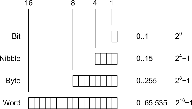
For inputs from things such as sensor switches, the size might be just a single bit. In other cases, such as when measuring analog data like pressure or temperature, the input might be converted into binary data values of 8, 10, 12, 16, or more bits in size. The number of available bits determines the range of numeric values that can be represented. Although it’s not shown in Figure 1-1, binary data can represent negative values as well as positive values, and there is a standard format for handling floating-point values as well.
Analog data, on the other hand, is continuously variable and may take on any value within a range of valid values. For example, consider the set of all possible floating-point values in the range between 0 and 1. One might find numbers like 0.01, 0.834, 0.59904041123, or 0.00000048, and anything in between. The name analog data is derived from the fact that the data is an analog of a continuously variable physical phenomenon.
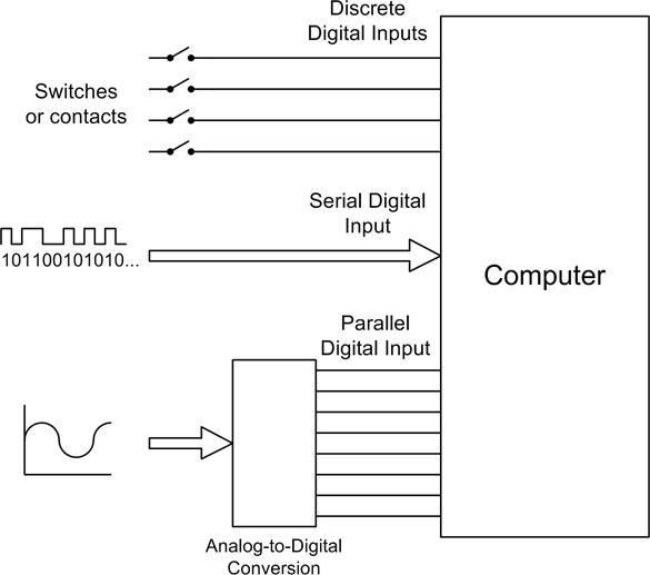
Figure 1-2 shows the various types of inputs that may be found in a computer-based data acquisition system. Switches are the equivalents of single binary digits (bits). A serial communications interface may be a single wire carrying a stream of bits end-to-end, where each set of 8 bits represents a single alphanumeric character, or perhaps a binary value. Analog input signals, in the form of a voltage or a current, are converted into digital values using a device called an analog-to-digital converter (ADC). We will take a close look at these devices—and their counterparts, digital-to-analog converters (DACs)—in Chapter 2.
Control Output
Whereas the data acquisition part of an instrumentation system senses the physical world and provides input data, the control part of an instrumentation system uses that data to effect changes in the physical world. Control of a physical device involves transforming some type of command or sensor input into a form suitable to cause a change in the activity of that device. More specifically, control entails generating digital or analog signals (or both) that may be used to perform a control action on a device or system. Linear control systems can be broadly grouped into two primary categories, open-loop and closed-loop, depending on whether or not they employ the concept of feedback.
Another common type of control system, the sequential control, utilizes time as its primary control input. In a sequential system, events occur at specific times relative to a primary event, and each event is typically discrete. In other words, a sequential event is either on or off, active or inactive. A computer is, by its very nature, a form of sequential controller, and sequential controls can usually be modeled using state machines. We’ll look at state diagrams in Chapter 8.
We will encounter all three types of control systems in this book. Chapter 9 goes into the theory behind them in more detail, but for now, a high-level overview will suffice to set the stage.
Open-Loop Control
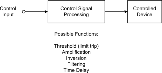
In an open-loop scheme, there is no feedback between the output and the control input of the system. In other words, the system has no way to determine if the control output actually had the desired effect. However, this doesn’t prevent it from being useful. The accuracy of an open-loop control system depends on the accuracy of its components and how well the system models what it is controlling. Figure 1-3 shows a simple block diagram of an open-loop control system. The block labeled “Controlled Device” might be an electric motor, a lamp, a fan, or a valve. While it might appear that there isn’t much going on here, open-loop controls can actually entail a high degree of complexity and they are fairly common.
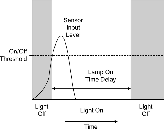
Even though an open-loop control system is “blind,” in a sense, it can still incorporate time into its design. An automatic light switch is one possible real-world example. A greatly simplified diagram of such a device is shown in Figure 1-4.
These popular devices contain a sensor (typically infrared) that will activate a floodlight if something appears in the field of view of the sensor. There is no feedback to ensure that the lights actually come on (at least, not in the typical units for residential use), nor can the sensor easily distinguish between a burglar and a large housecat.
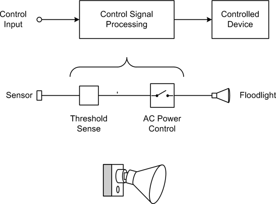
An automatic light does, however, have a built-in time delay to hold the light on for a period of time after the sensor’s input threshold has been crossed; otherwise, it would just turn on and then immediately turn back off again when the sensor input dropped back below the threshold. This is shown in the diagram in Figure 1-5. If there were no time delay to hold the lamp on, a large housecat hopping up and down in front of the sensor would cause the light to flash on and off repeatedly. This would probably annoy the neighbors (then again, automatic lights with excessive time delays can annoy the neighbors as well).
Closed-Loop Control
A closed-loop control scheme utilizes data obtained from the device or system under control, known as feedback, to determine the effect of the control and modify the control actions in accordance with some internal algorithm (also known as the “control laws”). Figure 1-6 shows a block diagram of a basic closed-loop control system.
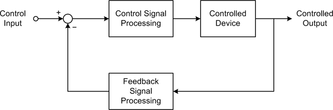
Notice that the control input and the feedback signal are summed with opposing signs at the circle symbol in Figure 1-6, which is called a “summing junction” or “summing node.” The output is called the control error. This is because the key to a closed-loop control is the response of the controlled device to the control signal generated by the block labeled “Control Signal Processing.” The control error is input to the control signal processing block, and the system will attempt to drive its control output into the controlled device to whatever extent is needed or possible in order to make the control error zero. Those readers who are familiar with operational amplifier (op amp) circuits will recognize this immediately: it’s the same principle that op amp circuits are based on.
As one might suspect, there is more going on here than the system diagram in Figure 1-6 shows. Both the control and feedback processing blocks may have some degree of amplification (gain) incorporated into their design. They may also include attenuation, filters, or limit thresholds. Gain levels are selected based on the application, and responses may even be nonlinear if necessary.
Here’s a somewhat more interesting closed-loop control example. Let’s assume that we want to maintain a constant fluid level in a storage tank while its contents are removed at varying rates. At some times the drain rate may be quite high, while at other times it may be very low or even zero. Figure 1-7 shows the setup and its associated control loop.
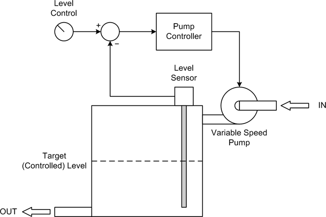
A sensor measures the fluid level in the tank, and if it is below the commanded value the rate of the input pump is commanded to increase so more fluid will enter the tank. As the fluid level approaches the target setting, the rate of the pump decreases, and once the target is reached it stops completely. This arrangement will automatically compensate for changes in how fast the fluid is drawn off from the tank, so long as the drain rate does not exceed the ability of the pump to keep up with it.
Sequential Control
Sequential controls are a very common form of control system and are straightforward to implement. Automated packaging systems, such as those used to form cereal boxes or fill plastic bags with animal feed, are typically timed sequential controls that perform specific actions using electrical or pneumatic actuators. Other sequential controls might employ some type of sensing to change sequences as necessary, or to sense a fault condition and halt the system.
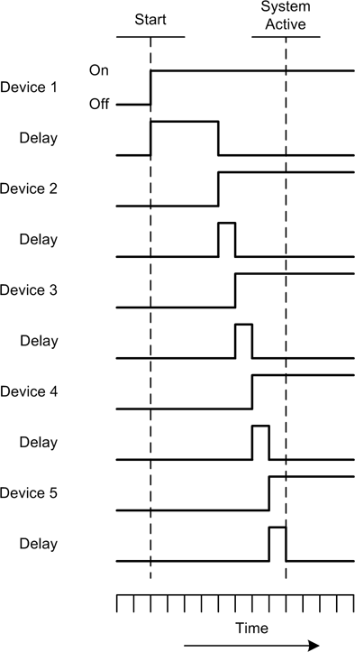
Figure 1-8 shows the timing diagram for a sequential AC power controller with five devices. In this example, a delay after each device is powered on allows it to stabilize and respond to a query to verify that it is functioning correctly. In a system such as this, each device would typically have three possible states: On, Off, and Fail. In addition to commanding the devices on or off in a timed sequence, the controller would also check each device to verify that it powered up correctly. Should a device fail, the controller would either halt the sequence or begin an automatic shutdown by disabling the devices already enabled, in reverse order.
Applications Overview
Let’s take a quick tour of some real-world examples of computer-based instrumentation applications. Please bear in mind that these examples are intended to show what one can do with automated instrumentation, not as specific, detailed examples of how to do something. In later chapters we will get into the specifics of interfaces, control protocols, and software algorithms.
Electronics Test Instrumentation
In an electronics laboratory, or even a well-equipped hobbyist’s workshop, it wouldn’t be unusual to encounter oscilloscopes, logic analyzers, frequency meters, signal generators, and other such devices. While these are useful devices in their own right, when incorporated into an automated system they can become even more useful.
In order to use a piece of test equipment in an automated setup, there must be some type of control or acquisition interface available. Many modern instruments incorporate USB, Ethernet, GPIB, RS-232, or a combination of these (these interfaces are examined in Chapters 7 and 11). In some cases, they are standard features; in other cases, the functionality must be ordered as a separate option when the instrument is purchased.
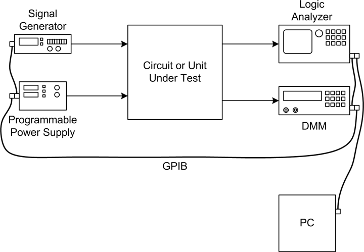
Figure 1-9 shows a simple arrangement for driving a device (the unit under test, or UUT) with a signal while controlling its DC power source, and acquiring measurement data in the form of logic analyzer traces and digital multimeter (DMM) readings.
The simple setup shown in Figure 1-9 has one instrument connected as a primary stimulus input to the UUT: namely, the signal generator. The signal it generates has a programmable shape (waveform) and rate (frequency). The signal level (amplitude) can also be controlled by the PC. There are two instruments connected to outputs from the UUT to capture digital logic signals (the logic analyzer) and one or more voltages (the DMM). A programmable power supply rounds out the instruments by providing a computer-controlled source of power to the UUT.
In this example, the various instruments are connected to the PC using a General Purpose Interface Bus (GPIB, also referred to as IEEE-488). There are various GPIB interface components available, ranging from plug-in PCI cards to external USB-to-GPIB adapters. Later in this book, we’ll examine some of these and look at various ways to write software for them in order to control instruments and collect data.
But what does it do? What Figure 1-9 shows could well be a performance characterization setup. If the UUT generates a pattern of digital signals in response to an input from the signal generator, this test arrangement will capture that behavior. It will also capture how the UUT’s behavior might change as the output from the programmable power supply is changed, or how some internal voltage might change as the frequency of the input from the signal generator changes. All of this data can be displayed on the PC’s monitor and captured to disk for storage and possible analysis at a later time.
Laboratory Instrumentation
A research laboratory might contain pH meters, temperature sensors, precision ovens, tunable lasers, and vacuum pumps (for starters). Figure 1-10 shows an example of an instrumentation system for controlling an environmental chamber.
For our purposes, it’s not really important what the chamber is used for (it could be used for microbe cultures, or perhaps for epoxy curing). What is important are the instruments connected to it and how they, in turn, are interfaced to the computer. Whereas in the previous example the instrument interface was implemented using GPIB, here we have plain old vanilla serial connections in the form of RS-232 interfaces.
The data acquisition instrument is responsible for sensing and converting analog signals such as temperature, and perhaps humidity. It might also monitor the electrical status of any heaters or coolers attached to the chamber. The power controller instrument is responsible for any heaters, coolers, cryogenic valves, or other controlled functions in the chamber.
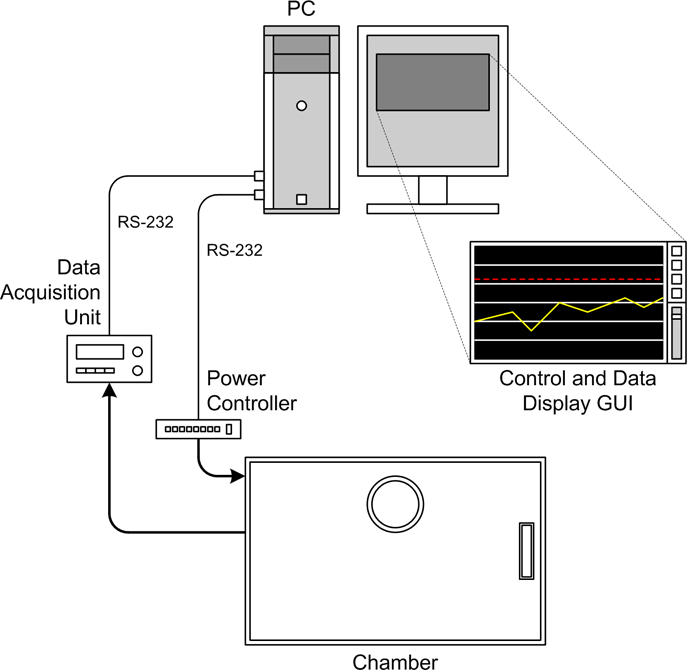
The primary objective of a setup such as this would probably be to maintain a specific temperature over time within some predefined range. It might also incorporate temperature ramp-up and ramp-down characteristics, depending on what exactly it is being used for. Generally, nothing in a system like this happens on a short time scale; significant changes may take anywhere from minutes to hours.
If implemented as a bang-bang controller, a type of on-off non-linear controller that we will look at in detail later on, there won’t be any need to vary the amount of power applied to the heaters or the cooling system. It operates much like the thermostat in a house. The instrumentation can utilize the rather slow RS-232 interfaces because there is no need to run the controller with a small time constant (i.e, a fast acquisition rate).
Process Control
The diagram in Figure 1-11 is a representation of a simple automated process control system. This system might be intended for producing artificial maple syrup, or it could be some other kind of controlled chemical reaction to produce a specific output product. Note that the diagram is somewhat nonstandard, mainly because its intent is to illustrate without getting wrapped up in the details of standardized process control symbology.
In Figure 1-11, we see yet another type of interface—the USB interface module. These are common and relatively inexpensive. You can even buy one as a kit if you feel inclined to build it yourself. Many provide a set of discrete inputs and outputs, some analog inputs with 10- or 12-bit conversion, and perhaps even some analog outputs or a pulse-width modulation (PWM) channel or two.
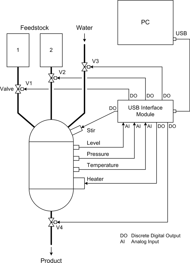
There are four valves in the diagram shown in Figure 1-11, labeled V1 through V4, each of which is connected to one of the discrete outputs from the USB interface module. A heater is also connected to a discrete output. Note that the diagram does not show any circuitry that might be necessary to convert the 5-volt discrete signal from the USB controller into something with enough current and/or voltage to drive the valves or the heater. We’ll examine how to drive external devices that utilize high currents or high voltages (or both) in Chapter 2. Three analog inputs are used to acquire liquid level, temperature, and pressure data from sensors.
As with the previous example, this probably would not be a high-speed system. It would most likely perform just fine if the sensors were read and the controls (valves and heater) updated every 1 to 5 seconds.
Summary
The domain of instrumentation applications is both broad and deep, and there is no way that a single chapter like this could possibly capture more than just a glimpse of what it is and what is possible. Some of the terms and concepts may have seemed new and strange, but they will be covered again in later chapters. The main goal here was to give you some exposure to the basic concepts. We’ll fill in the details as we go along.
Get Real World Instrumentation with Python now with the O’Reilly learning platform.
O’Reilly members experience books, live events, courses curated by job role, and more from O’Reilly and nearly 200 top publishers.

