9.6 Appendix 9.1: Parametric Estimation Using Second Derivatives
We now go through an example of using second derivatives for parametric estimation, as laid out in the appendix of Chapter 8. As discussed there, second derivatives can be used with an asymptotic Cornish-Fisher expansion for the inverse CDF to provide a flag for when nonlinearities are large enough to make a difference in quantile (VaR) estimation.
For parametric or linear estimation (for a single risk factor, using first derivatives only and assuming μ = 0) the portfolio mean and variance are:
1st moment: zero
2nd moment: δ2σ2
Using second derivatives, the first four central moments are:
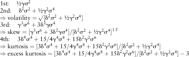
We can examine this for the $20M position in the 10-year U.S. Treasury. A bond is a reasonably linear asset and so we should expect no nonlinear effects from including the second derivatives. The delta and gamma (first and second derivative, or DV01 and convexity) are:
![]()
while the volatility of yields is 7.15bp per day. This gives the following moments:
| Linear | Quadratic | |
| Mean | 0.0 | 450 |
| Volatility | 130,789 | 130,791 |
| Skew | 0.0 | 0.0206 |
| Excess Kurtosis | 0.0 | 0.0006 |
The skew and kurtosis are so small they clearly will have no discernible impact on the shape of the P&L distribution.
In contrast, an option will have considerable nonlinearity ...
Get Quantitative Risk Management: A Practical Guide to Financial Risk, + Website now with the O’Reilly learning platform.
O’Reilly members experience books, live events, courses curated by job role, and more from O’Reilly and nearly 200 top publishers.

