Chapter 4. How Chunking and Compression Can Help You
So far we have avoided talking about exactly how the data you write is stored on disk. Some of the most interesting features in HDF5, including per-dataset compression, are tied up in the details of how data is arranged on disk.
Before we get down to the nuts and bolts, there’s a more fundamental issue we have to discuss: how multidimensional arrays are actually handled in Python and HDF5.
Contiguous Storage
Let’s suppose we have a four-element NumPy array of strings:
>>>a=np.array([["A","B"],["C","D"]])>>>a[['A' 'B']['C' 'D']]
Mathematically, this is a two-dimensional object. It has two axes, and can be indexed using a pair of numbers in the range 0 to 1:
>>>a[1,1]'D'
However, there’s no such thing as “two-dimensional” computer memory, at least not in common use. The elements are actually stored in a one-dimensional buffer:
'A''B''C''D'
This is called contiguous storage, because all the elements of the array, whether it’s stored on disk or in memory, are stored one after another. NumPy uses a simple set of rules to turn an indexing expression into the appropriate offset into this one-dimensional buffer. In this case, indexing along the first axis advances us into the buffer in steps (strides, in NumPy lingo) of 2, while indexing along the second axis advances us in steps of 1.
For example, the indexing expression a[0,1] is handled as follows:
offset = 2*0 + 1*1 -> 1
buffer[offset] -> value "B"
Note
You might notice that there are two possible conventions here: whether the “fastest-varying” index is the last (as previously shown), or the first. This choice is the difference between row-major and column-major ordering. Python, C, and HDF5 all use row-major ordering, as in the example.
By default, all but the smallest HDF5 datasets use contiguous storage. The data in your dataset is flattened to disk using the same rules that NumPy (and C, incidentally) uses.
If you think about it, this means that certain operations are much faster than others. Consider as an example a dataset containing one hundred 640×480 grayscale images. Let’s say the shape of the dataset is (100, 480, 640):
>>>f=h5py.File("imagetest.hdf5")>>>dset=f.create_dataset("Images",(100,480,640),dtype='uint8')
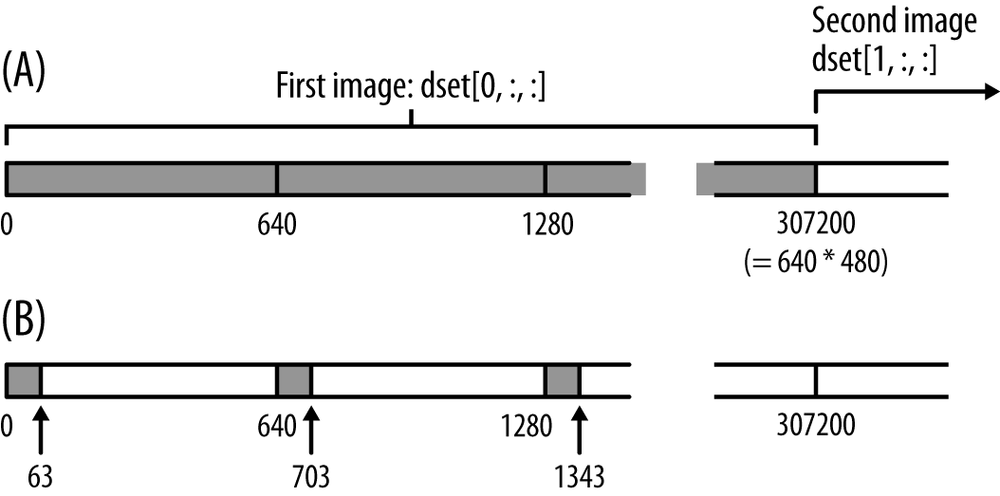
A contiguous dataset would store the image data on disk, one 640-element “scanline” after another. If we want to read the first image, the slicing code would be:
>>>image=dset[0,:,:]>>>image.shape(480, 640)
Figure 4-1(A) shows how this works. Notice that data is stored in “blocks” of 640 bytes that correspond to the last axis in the dataset. When we read in the first image, 480 of these blocks are read from disk, all in one big block.
This leads us to the first rule (really, the only one) for dealing with data on disk, locality: reads are generally faster when the data being accessed is all stored together. Keeping data together helps for lots of reasons, not the least of which is taking advantage of caching performed by the operating system and HDF5 itself.
It’s easy to see that applications reading a whole image, or a series of whole images, will be efficient at reading the data. The advantage of contiguous storage is that the layout on disk corresponds directly to the shape of the dataset: stepping through the last index always means moving through the data in order on disk.
But what if, instead of processing whole images one after another, our application deals with image tiles? Let’s say we want to read and process the data in a 64×64 pixel slice in the corner of the first image; for example, say we want to add a logo.
Our slicing selection would be:
>>>tile=dset[0,0:64,0:64]>>>tile.shape(64, 64)
Figure 4-1(B) shows how the data is read in this case.
Not so good. Instead of reading one nice contiguous block of data, our
application has to gather data from all over the place. If we wanted the 64×64
tile from every image at once (dset[:,0:64,0:64]), we’d have to read all the
way to the end of the dataset!
The fundamental problem here is that the default contiguous storage mechanism does not match our access pattern.
Chunked Storage
What if there were some way to express this in advance? Isn’t there a way to preserve the shape of the dataset, which is semantically important, but tell HDF5 to optimize the dataset for access in 64×64 pixel blocks?
That’s what chunking does in HDF5. It lets you specify the N-dimensional “shape” that best fits your access pattern. When the time comes to write data to disk, HDF5 splits the data into “chunks” of the specified shape, flattens them, and writes them to disk. The chunks are stored in various places in the file and their coordinates are indexed by a B-tree.
Here’s an example. Let’s take the (100, 480, 640)-shape dataset just shown and
tell HDF5 to store it in chunked format. We do this by providing a new
keyword, chunks, to the create_dataset method:
>>>dset=f.create_dataset('chunked',(100,480,640),dtype='i1',chunks=(1,64,64))
Like a dataset’s type, this quantity, the chunk shape, is fixed when the
dataset is created and can never be changed. You can check the chunk shape
by inspecting the chunks property; if it’s None, the dataset isn’t using
chunked storage:
>>>dset.chunks(1, 64, 64)
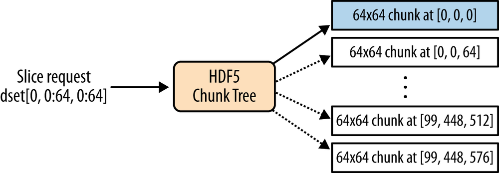
The chunk shape always has the same number of elements as the dataset shape; in this example, three. Let’s repeat the 64×64-pixel slice, as before:
>>>dset[0,0:64,0:64]
Figure 4-2 shows how this is handled. Much better. In this example, only one chunk is needed; HDF5 tracks it down and reads it from disk in one continuous lump.
Even better, since chunked data is stored in nice uniformly sized packets of bytes, you can apply all kinds of operations to it when writing or reading from the file. For example, this is how compression works in HDF5; on their way to and from the disk, chunks are run through a compressor or decompressor. Such filters in HDF5 (see Filters and Compression) are completely transparent to the reading application.
Keep in mind that chunking is a storage detail only. You don’t need to do anything special to read or write data in a chunked dataset. Just use the normal NumPy-style slicing syntax and let HDF5 deal with the storage.
Setting the Chunk Shape
You are certainly free to pick your own chunk shape, although be sure to read about the performance implications later in this chapter. Most of the time, chunking will be automatically enabled by using features like compression or marking a dataset as resizable. In that case, the auto-chunker in h5py will help you pick a chunk size.
Auto-Chunking
If you don’t want to sit down and figure out a chunk shape, you can have h5py
try to guess one for you by setting chunks to True instead of a tuple:
>>>dset=f.create_dataset("Images2",(100,480,640),'f',chunks=True)>>>dset.chunks(13, 60, 80)
The “auto-chunker” tries to keep chunks mostly “square” (in N dimensions) and within certain size limits. It’s also invoked when you specify the use of compression or other filters without explicitly providing a chunk shape.
By the way, the reason the automatically generated chunks are “square” in N dimensions is that the auto-chunker has no idea what you’re planning to do with the dataset, and is hedging its bets. It’s ideal for people who just want to compress a dataset and don’t want to bother with the details, but less ideal for those with specific time-critical access patterns.
Manually Picking a Shape
Here are some things to keep in mind when working with chunks. The process of picking a chunk shape is a trade-off between the following three constraints:
- Larger chunks for a given dataset size reduce the size of the chunk B-tree, making it faster to find and load chunks.
- Since chunks are all or nothing (reading a portion loads the entire chunk), larger chunks also increase the chance that you’ll read data into memory you won’t use.
- The HDF5 chunk cache can only hold a finite number of chunks. Chunks bigger than 1 MiB don’t even participate in the cache.
So here are the main points to keep in mind:
- Do you even need to specify a chunk size?
- It’s best to restrict manual chunk sizing to cases when you know for sure your dataset will be accessed in a way that’s likely to be inefficient with either contiguous storage or an auto-guessed chunk shape. And like all optimizations, you should benchmark!
- Try to express the “natural” access pattern your dataset will have
- As in our example, if you are storing a bunch of images in a dataset and know that your application will be reading particular 64×64 “tiles,” you could use N×64×64 chunks (or N×128×128) along the image axes.
- Don’t make them too small
- Keep in mind that HDF5 has to use indexing data to keep track of things; if you use something pathological like a 1-byte chunk size, most of your disk space will be taken up by metadata. A good rule of thumb for most datasets is to keep chunks above 10KiB or so.
- Don’t make them too big
- The key thing to remember is that when you read any data in a chunk, the entire chunk is read. If you only use a subset of the data, the extra time spent reading from disk is wasted. Keep in mind that chunks bigger than 1 MiB by default will not participate in the fast, in-memory “chunk cache” and will instead be read from disk every time.
Performance Example: Resizable Datasets
In the last example of Chapter 3, we discussed some of the performance aspects of resizable datasets. It turns out that with one or two exceptions, HDF5 requires that resizable datasets use chunked storage. This makes sense if you think about how contiguous datasets are stored; expanding any but the last axis would require rewriting the entire dataset!
There are some chunk-related pitfalls when using resizable datasets, one of which illustrates why you have to be careful of using the auto-chunker where performance is critical. It may make decisions that don’t match your idea of how the dataset will be used.
Revisiting the example in Chapter 3, let’s create two datasets to store a collection of 1000-element-long time traces. The datasets will both be created as expandable along their first axes, and differ only in their initial sizes:
>>>dset1=f.create_dataset('timetraces1',(1,1000),maxshape=(None,1000))>>>dset2=f.create_dataset('timetraces2',(5000,1000),maxshape=(None,1000))
Recall that we had two different approaches to “appending” data to these arrays:
simple appending (add_trace_1) and overallocate-and-trim
(add_trace_2 and done). The second approach was supposed to be faster, as
it involved fewer calls to resize:
defadd_trace_1(arr):""" Add one trace to the dataset, expanding it as necessary """dset1.resize((dset1.shape[0]+1,1000))dset1[-1,:]=arrntraces=0defadd_trace_2(arr):""" Add one trace to the dataset, keeping count of the # of traceswritten """globalntracesdset2[ntraces,:]=arrntraces+=1defdone():""" After all calls to add_trace_2, trim the dataset to size """dset2.resize((ntraces,1000))
Now, let’s actually test the performance with timeit:
defsetup():""" Re-initialize both datasets for the tests """globaldata,N,dset1,dset2,ntracesdata=np.random.random(1000)N=10000# Number of iterationsdset1.resize((1,1000))dset2.resize((10001,1000))ntraces=0deftest1():""" Add N traces to the first dataset """foridxinxrange(N):add_trace_1(data)deftest2():""" Add N traces to the second dataset, and then trim it """foridxinxrange(N):add_trace_2(data)done()
>>>timeit(test1,setup=setup,number=1)3.0431830883026123>>>timeit(test2,setup=setup,number=1)3.3972668647766113
Not quite what we expected. What’s going on? One clue comes from inspecting the chunk shape for each dataset:
>>>dset1.chunks(1, 1000)>>>dset2.chunks(63, 125)
What happened? It turns out that the chunk shape is determined by, among other things, the initial size of the dataset. Let’s manually specify a chunk shape and try again. This time we’ll set both of them to a shape of (1, 1000), giving us 4k chunks in both cases (1000 elements × 4 bytes):
>>>dset1=f.create_dataset('timetraces3',(1,1000),maxshape=(None,1000),chunks=(1,1000))>>>dset2=f.create_dataset('timetraces4',(5000,1000),maxshape=(None,1000),chunks=(1,1000))>>>timeit(test1,setup=setup,number=1)3.0520598888397217>>>timeit(test2,setup=setup,number=1)2.5036721229553223
Much better. Next, we explore the “killer app” for chunks, arguably even more important than their role in boosting performance: filters.
Filters and Compression
If you wanted to compress a contiguous dataset, you would quickly realize that the entire thing would have to be decompressed and recompressed every time you wrote an element. That’s because there’s no simple way to index into a compressed dataset using offsets, like you can with an uncompressed contiguous dataset. After all, the point of compression is that you end up with a variable-sized output depending on the values involved.
With chunking, it becomes possible to transparently perform compression on a dataset. The initial size of each chunk is known, and since they’re indexed by a B-tree they can be stored anywhere in the file, not just one after another. In other words, each chunk is free to grow or shrink without banging into the others.
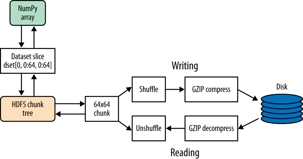
The Filter Pipeline
HDF5 has the concept of a filter pipeline, which is just a series of operations performed on each chunk when it’s written. Each filter is free to do anything it wants to the data in the chunk: compress it, checksum it, add metadata, anything. When the file is read, each filter is run in “reverse” mode to reconstruct the original data.
Figure 4-3 shows schematically how this works. You’ll notice that since the atomic unit of data here is the chunk, reading or writing any data (even a single element) will result in decompression of at least one entire chunk. This is one thing to keep in mind when selecting a chunk shape, or choosing whether compression is right for your application.
Finally, you have to specify your filters when the dataset is created, and they can never change.
Compression Filters
A number of compression filters are available in HDF5. By far the most commonly used is the GZIP filter. (You’ll also hear this referred to as the “DEFLATE” filter; in the HDF5 world both names are used for the same filter.)
Here’s an example of GZIP compression used on a floating-point dataset:
>>>dset=f.create_dataset("BigDataset",(1000,1000),dtype='f',compression="gzip")>>>dset.compression'gzip'
By the way, you’re not limited to floats. The great thing about GZIP compression is that it works with all fixed-width HDF5 types, not just numeric types.
Compression is transparent; data is read and written normally:
>>>dset[...]=42.0>>>dset[0,0]42.0
Investigating the Dataset object, we find a few more properties:
>>>dset.compression_opts4>>>dset.chunks(63, 125)
The compression_opts property (and corresponding keyword to create_dataset)
reflects any settings for the compression filter. In this case, the default
GZIP level is 4.
You’ll notice that the auto-chunker has selected a chunk shape for us: (63, 125).
Data is broken up into chunks of 63*125*(4 bytes) = 30KiB blocks for the
compressor.
The following sections cover some of the available compression filters, and details about each.
GZIP/DEFLATE Compression
As we just saw, GZIP compression is by far the simplest and most portable compressor in HDF5. It ships with every installation of HDF5, and has the following benefits:
- Works with all HDF5 types
- Built into HDF5 and available everywhere
- Moderate to slow speed compression
- Performance can be improved by also using SHUFFLE (see SHUFFLE Filter)
For the GZIP compressor, compression_opts may be an integer from 0 to 9,
with a default of 4.
>>>dset=f.create_dataset("Dataset",(1000,),compression="gzip")
It’s also invoked if you specify a number as the argument to compression:
>>>dset=f.create_dataset("Dataset2",(1000,),compression=9)>>>dset.compression'gzip'>>>dset.compression_opts9
SZIP Compression
SZIP is a patented compression technology used extensively by NASA. Generally you only have to worry about this if you’re exchanging files with people who use satellite data. Because of patent licensing restrictions, many installations of HDF5 have the compressor (but not the decompressor) disabled.
>>>dset=myfile.create_dataset("Dataset3",(1000,),compression="szip")
SZIP features:
- Integer (1, 2, 4, 8 byte; signed/unsigned) and floating-point (4/8 byte) types only
- Fast compression and decompression
- A decompressor that is almost always available
LZF Compression
For files you’ll only be using from Python, LZF is a good choice. It ships
with h5py; C source code is available for third-party programs under the BSD
license. It’s optimized for very, very fast compression at the expense of
a lower compression ratio compared to GZIP. The best use case for this is
if your dataset has large numbers of redundant data points. There are no
compression_opts for this filter.
>>>dset=myfile.create_dataset("Dataset4",(1000,),compression="lzf")
LZF compression:
- Works with all HDF5 types
- Features fast compression and decompression
- Is only available in Python (ships with h5py); C source available
Performance
As always, you should run your own performance tests to see what parts of your application would benefit from attention. However, here are some examples to give you an idea of how the various filters stack up. In this experiment (see h5py.org/lzf for details), a 4 MB dataset of single-precision floats was tested against the LZF, GZIP, and SZIP compressors. A 190 KiB chunk size was used.
First, the data elements were assigned their own indices (see Table 4-1):
>>>data[...]=np.arange(1024000)
| Compressor | Compression time (ms) | Decompression time (ms) | Compressed by |
None | 10.7 | 6.5 | 0.00% |
LZF | 18.6 | 17.8 | 96.66% |
GZIP | 58.1 | 40.5 | 98.53% |
SZIP | 63.1 | 61.3 | 72.68% |
Next, a sine wave with added noise was tested (see Table 4-2):
>>>data[...]=np.sin(np.arange(1024000)/32.)+(np.random(1024000)*0.5-0.25)
| Compressor | Compression time (ms) | Decompression time (ms) | Compressed by |
None | 10.8 | 6.5 | 0.00% |
LZF | 65.5 | 24.4 | 15.54% |
GZIP | 298.6 | 64.8 | 20.05% |
SZIP | 115.2 | 102.5 | 16.29% |
Finally, random float values were used (see Table 4-3):
>>>data[...]=np.random(1024000)
| Compressor | Compression time (ms) | Decompression time (ms) | Compressed by |
None | 9.0 | 7.8 | 0.00% |
LZF | 67.8 | 24.9 | 8.95% |
GZIP | 305.4 | 67.2 | 17.05% |
SZIP | 120.6 | 107.7 | 15.56% |
Again, don’t take these figures as gospel. Other filters (BLOSC, for example, see Third-Party Filters) are even faster than LZF. It’s also rare for an application to spend most of its time compressing or decompressing data, so try not to get carried away with speed testing.
Other Filters
HDF5 includes some extra goodies like consistency check filters and a rearrangement (SHUFFLE) filter to boost compression performance. These filters, and any compression filters you specify, are assembled by HDF5 into the filter pipeline and run one after another.
SHUFFLE Filter
This filter is only ever used in conjunction with a compression filter like GZIP or LZF. It exploits the fact that, for many datasets, most of the entropy occurs in only a few bytes of the type. For example, if you have a 4-byte unsigned integer dataset but your values are generally zero to a few thousand, most of the data resides in the lower two bytes. The first three integers of a dataset might look like this (big-endian format):
(0x00 0x00 0x02 0x3E) (0x00 0x00 0x01 0x42) (0x00 0x00 0x01 0x06) ...
The SHUFFLE filter repacks the data in the chunk so that all the first bytes of the integers are together, then all the second bytes, and so on. So you end up with a chunk like this:
(0x00 0x00 0x00 ... ) (0x00 0x00 0x00 ... ) (0x02 0x01 0x01 ... ) (0x3E 0x42 0x06 ...)
For dictionary-based compressors like GZIP and LZF, it’s much more efficient to compress long runs of identical values, like all the zero values collected from the first two bytes of the dataset’s integers. There are also savings from the repeated elements at the third byte position. Only the fourth byte position looks really hard to compress.
Here’s how to enable the SHUFFLE filter (in conjunction with GZIP):
>>>dset=myfile.create_dataset("Data",(1000,),compression="gzip",shuffle=True)
To check if a dataset has SHUFFLE enabled, use the following:
>>>dset.shuffleTrue
The SHUFFLE filter is:
- Available with all HDF5 distributions
- Very, very fast (negligible compared to the compression time)
- Only useful in conjunction with filters like GZIP or LZF
FLETCHER32 Filter
Accidents happen. When you’re storing or transmitting a multiterabyte dataset, you’d like to be sure that the bytes that come out of the file are the same ones you put in. HDF5 includes a checksum filter for just this purpose. It uses a 32-bit implementation of Fletcher’s checksum, hence the name FLETCHER32.
A checksum is computed when each chunk is written to the file, and recorded in the chunk’s metadata. When the chunk is read, the checksum is computed again and compared to the old one. If they don’t match, an error is raised and the read fails.
Here’s how to enable checksumming for a new dataset:
>>>dset=myfile.create_dataset("Data2",(1000,),fletcher32=True)
To see if a dataset has checksumming enabled, use the following:
>>>dset.fletcher32True
The FLETCHER32 filter is:
- Available with all HDF5 distributions
- Very fast
- Compatible with all lossless filters
Third-Party Filters
Many other filters exist for HDF5. For example, the BLOSC compressor used by the PyTables project is highly tuned for speed. Other filters also exist that are based on the LZO compression system, BZIP2, and more. You can find the most recent list (and contact information for the filter developers) at the HDF Group website.
There’s one more thing to mention, and it’s a very new feature (introduced in HDF5 1.8.11): dynamically loaded filters. For the filters listed previously, you have to manually “register” them with the HDF5 library before they can be used. For example, h5py registers the LZF filter when it starts up. Newer versions of HDF5 will automatically load filter modules from disk when they encounter an unknown filter type in a dataset. Dynamic loading is a new technology in HDF5 and support for it in h5py and PyTables is still evolving. Your best bet is to check the h5py and PyTables websites for the most up-to-date information.
And one final reminder: when you use a filter, be sure the people you intend to share the data with also have access to it.
Get Python and HDF5 now with the O’Reilly learning platform.
O’Reilly members experience books, live events, courses curated by job role, and more from O’Reilly and nearly 200 top publishers.

