In the previous chapter we worked through the basics of Pig Latin. In this chapter we will plumb its depths, and we will also discuss how Pig handles more complex data flows. Finally, we will look at how to use macros and modules to modularize your scripts.
We will now discuss the more advanced Pig Latin operators, as well as additional options for operators that were introduced in the previous chapter.
In our introduction to foreach (see foreach), we discussed how it could take a list of
expressions to output for every record in your data pipeline. Now we
will look at ways it can explode the number of records in your pipeline,
and also how it can be used to apply a set of operations to each
record.
Sometimes you have data in a bag or a tuple and you want
to remove that level of nesting. The baseball data
available on GitHub (see Code Examples in This Book) can be used
as an example. Because a player can play more than one position,
position is stored in a bag. This allows us to
still have one entry per player in the baseball file.[15] But when you want to switch around your data on the fly
and group by a particular position, you need a way to pull those
entries out of the bag. To do this, Pig provides the
flatten modifier in foreach:
--flatten.pig
players = load 'baseball' as (name:chararray, team:chararray,
            position:bag{t:(p:chararray)}, bat:map[]);
pos     = foreach players generate name, flatten(position) as position;
bypos   = group pos by position;
A foreach with a
flatten produces a cross product of every record in the
bag with all of the other expressions in the generate
statement. Looking at the first record in baseball, we see it is the following
(replacing tabs with commas for clarity):
Jorge Posada,New York Yankees,{(Catcher),(Designated_hitter)},...
Once this has passed through the
flatten statement, it will be two records:
Jorge Posada,Catcher

Jorge Posada,Designated_hitter
If there is more than one bag and both are
flattened, this cross product will be done with members of each bag as
well as other expressions in the generate statement. So
rather than getting n rows (where
n is the number of records in one
bag), you will get n * m
rows.
One side effect that surprises many users is
that if the bag is empty, no records are produced. So if there had
been an entry in baseball with no
position, either because the bag is null or empty, that record would
not be contained in the output of flatten.pig. The record with the empty bag
would be swallowed by foreach. There are a couple of
reasons for this behavior. One, since Pig may or may not have the
schema of the data in the bag, it might have no idea how to fill in
nulls for the missing fields. Two, from a mathematical perspective,
this is what you would expect. Crossing a set S with the empty set results in the empty
set. If you wish to avoid this, use a bincond to replace empty bags
with a constant bag:
--flatten_noempty.pig
players = load 'baseball' as (name:chararray, team:chararray,
            position:bag{t:(p:chararray)}, bat:map[]);
noempty = foreach players generate name,
            ((position is null or IsEmpty(position)) ? {('unknown')} : position)
            as position;
pos     = foreach noempty generate name, flatten(position) as position;
bypos   = group pos by position;
flatten can also be applied to a
tuple. In this case, it does not produce a cross product; instead, it
elevates each field in the tuple to a top-level field. Again, empty
tuples will remove the entire record.
If the fields in a bag or tuple that is being
flattened have names, Pig will carry those names along. As with
join, to avoid ambiguity, the field name will have
the bag’s name and :: prepended to
it. As long as the field name is not ambiguous, you are not required
to use the bagname:: prefix.
If you wish to change the names of the fields,
or if the fields initially did not have names, you can attach an
as clause to your flatten, as in the
preceding example. If there is more than one field in the bag or tuple
that you are assigning names to, you must surround the set of field
names with parentheses.
Finally, if you flatten a bag or tuple without
a schema and do not provide an as clause, the resulting
records coming out of your foreach will have a null
schema. This is because Pig will not know how many fields the
flatten will result in.[16]
So far, all of the examples of foreach that
we have seen immediately generate one or more lines of output. But
foreach is more powerful than this. It can also apply a
set of relational operations to each record in your pipeline. This is
referred to as a nested foreach, or inner
foreach. One example of how this can be used is to find the number of
unique entries in a group. For example, to find the number of
unique stock symbols for each exchange in the NYSE_daily data:
--distinct_symbols.pig
daily    = load 'NYSE_daily' as (exchange, symbol); -- not interested in other fields
grpd     = group daily by exchange;
uniqcnt  = foreach grpd {
           sym      = daily.symbol;
           uniq_sym = distinct sym;
           generate group, COUNT(uniq_sym);
};
There are several new things here to unpack;
we will walk through each. In this example, rather than
generate immediately following foreach, a
{ (open brace) signals that we will
be nesting operators inside this foreach. In this nested
code, each record passed to foreach is handled one at a
time.
In the first line we see a syntax that we have
not seen outside of foreach. In fact, sym =
daily.symbol would not be legal outside of
foreach. It is roughly equivalent to the top-level
statement sym = foreach grpd generate daily.symbol, but
it is not stated that way inside the foreach
because it is not really another foreach. There is no
relation for it to be associated with (that is, grpd is not defined here). This line takes
the bag daily and produces a new
relation sym, which is a bag with
tuples that have only the field symbol.
The second line applies the distinct operator to the relation
sym. Note that even inside
foreach, relational operators can be applied only to
relations; they cannot be applied to expressions. For example, the
statement uniq_sym = distinct daily.symbol will produce a
syntax error because daily.symbol
is an expression, not a relation. sym is a relation. This distinction may seem
arbitrary, but it results in Pig Latin having a coherent definition as a language.
Without this, strange statements such as C = distinct 1 +
2 would be legal. One way to think about this is that the
assignment operator inside foreach can be used to take an
expression and create a relation, as happens in this example.
The last line in a nested foreach
must always be generate. This tells Pig how to take the
results of the nested operations and produce a record to be put in the
outer relation (in this case, uniqcnt). So, generate is the
operator that takes the inner relations and turns them back into
expressions for inclusion in the outer relation. That is, if the
script read generate group, uniq_sym, uniq_sym would be treated as a bag for the
purpose of the generate statement.
Theoretically, any Pig Latin relational
operator should be legal inside foreach. However, at the
moment, only distinct, filter, limit, and order are supported.
Let’s look at a few more examples of how this feature can be useful, such as to sort the contents of a bag before the bag is passed to a UDF. This is convenient for UDFs that require all of their input to come in a certain order. Consider a stock-analysis UDF that wants to track information about a particular stock over time. The UDF will want input sorted by timestamp:
--analyze_stock.pig
register 'acme.jar';
define analyze com.acme.financial.AnalyzeStock();
daily    = load 'NYSE_daily' as (exchange:chararray, symbol:chararray,
               date:chararray, open:float, high:float, low:float,
               close:float, volume:int, adj_close:float);
grpd     = group daily by symbol;
analyzed = foreach grpd {
            sorted = order daily by date;
            generate group, analyze(sorted);
};
Doing the sorting in Pig Latin, rather than in
your UDF, is important for a couple of reasons. One, it means Pig can
offload the sorting to MapReduce. MapReduce has the ability to sort
data by a secondary key while grouping it. So, the order
statement in this case does not require a separate sorting operation.
Two, it means that your UDF does not need to wait for all data to be
available before it starts processing. Instead, it can use the
Accumulator interface (see Accumulator Interface), which is much more memory
efficient.
This feature can be used to find the top k elements in a group. The following example will find the top three dividends payed for each stock:
--hightest_dividend.pig
divs = load 'NYSE_dividends' as (exchange:chararray, symbol:chararray,
            date:chararray, dividends:float);
grpd = group divs by symbol;
top3 = foreach grpd {
            sorted = order divs by dividends desc;
            top    = limit sorted 3;
            generate group, flatten(top);
};
Currently, these nested portions of code are
always run serially for each record handed to them. Of course the
foreach itself will be running in multiple map or reduce
tasks, but each instance of the foreach will not spawn
subtasks to do the nested operations in parallel. So if we added a
parallel 10 clause to the grpd = group divs by
symbol statement in the previous example, this ordering and
limiting would take place in 10 reducers. But each group of stocks
would be sorted and the top three records taken serially within one of
those 10 reducers.
There is, of course, no requirement that the
pipeline inside the foreach be a simple linear pipeline.
For example, if you wanted to calculate two distinct counts together,
you could do the following:
--double_distinct.pig
divs = load 'NYSE_dividends' as (exchange:chararray, symbol:chararray);
grpd = group divs all;
uniq = foreach grpd {
            exchanges      = divs.exchange;
            uniq_exchanges = distinct exchanges;
            symbols        = divs.symbol;
            uniq_symbols   = distinct symbols;
            generate COUNT(uniq_exchanges), COUNT(uniq_symbols);
};
For simplicity, Pig actually runs this
pipeline once for each expression in generate. Here this
has no side effects because the two data flows are completely
disjointed. However, if you constructed a pipeline where there was a
split in the flow, and you put a UDF in the shared portion, you would
find that it was invoked more often than you expected.
When we covered join in the previous chapter
(see Join), we discussed only the default join
behavior. However, Pig offers multiple join implementations, which we
will discuss here.
In RDBMS systems, traditionally the SQL optimizer chooses a join implementation for the user.
This is nice as long as the optimizer chooses well, which it does in
most cases. But Pig has taken a different approach. In the Pig team we
like to say that our optimizer is located between the user’s chair and
keyboard. We empower the user to make these choices rather than having
Pig make them. So for operators such as join where there
are multiple implementations, Pig lets the user indicate his choice via
a using clause.
This approach fits well with our philosophy that Pigs are domestic animals (i.e., Pig does what you tell it; see Pig Philosophy). Also, as a relatively new product, Pig has a lot of functionality to add. It makes more sense to focus on adding implementation choices and letting the user choose which ones to use, rather than focusing on building an optimizer capable of choosing well.
A common type of join is doing a lookup in a smaller input. For example, suppose you were processing data where you needed to translate a US ZIP code (postal code) to the state and city it referred to. As there are at most 100,000 zip codes in the US, this translation table should easily fit in memory. Rather than forcing a reduce phase that will sort your big file plus this tiny zip code translation file, it makes sense instead to send the zip code file to every machine, load it into memory, and then do the join by streaming through the large file and looking up each record in the zip code file. This is called a fragment-replicate join (because you fragment one file and replicate the other):
--repljoin.pig
daily = load 'NYSE_daily' as (exchange:chararray, symbol:chararray,
            date:chararray, open:float, high:float, low:float,
            close:float, volume:int, adj_close:float);
divs  = load 'NYSE_dividends' as (exchange:chararray, symbol:chararray,
            date:chararray, dividends:float);
jnd   = join daily by (exchange, symbol), divs by (exchange, symbol)
            using 'replicated';
The using 'replicated' tells Pig
to use the fragment-replicate algorithm to execute this join. Because
no reduce phase is necessary, all of this can be done in the map
task.
The second input listed in the join (in this
case, divs) is always the input
that is loaded into memory. Pig does not check beforehand that the
specified input will fit into memory. If Pig cannot fit the replicated
input into memory, it will issue an error and fail.
Warning
Due to the way Java stores objects in memory, the size of the data on disk will not be the size of the data in memory. See Memory Requirements of Pig Data Types for a discussion of how data expands in memory in Pig. You will need more memory for a replicated join than you need space on disk to store the replicated input.
Fragment-replicate join supports only inner and left outer joins. It cannot do a right outer join, because when a given map task sees a record in the replicated input that does not match any record in the fragmented input, it has no idea whether it would match a record in a different fragment. So, it does not know whether to emit a record. If you want a right or full outer join, you will need to use the default join operation.
Fragment-replicate join can be used with more than two tables. In this case, all but the first (left-most) table are read into memory.
Pig implements the fragment-replicate join by loading the replicated input into Hadoop’s distributed cache. The distributed cache is a tool provided by Hadoop that preloads a file onto the local disk of nodes that will be executing the maps or reduces for that job. This has two important benefits. First, if you have a fragment-replicate join that is going to run on 1,000 maps, opening one file in HDFS from 1,000 different machines all at once puts a serious strain on the NameNode and the three data nodes that contain the block for that file. The distributed cache is built specifically to manage these kinds of issues without straining HDFS. Second, if multiple map tasks are located on the same physical machine, the files in the distributed cache are shared between those instances, thus reducing the number of times the file has to be copied.
Pig runs a map-only MapReduce job to
preprocess the file and get it ready for loading into the distributed
cache. If there is a filter or foreach
between the load and join, these will be
done as part of this initial job so that the file to be stored in the
distributed cache is as small as possible. The join itself will be
done in a second map-only job.
As we have seen elsewhere, much of the data you will be
processing with Pig has significant skew in the number of records per
key. For example, if you were building a map of the Web and joining by
the domain of the URL (your key), you would expect to see significant
skew for values such as yahoo.com.
Pig’s default join algorithm is very sensitive to skew, because it
collects all of the records for a given key together on a single
reducer. In many data sets, there are a few keys that
have three or more orders of magnitude more records than other keys.
This results in one or two reducers that will take much longer than
the rest. To deal with this, Pig provides skew
join.
Skew join works by first sampling one input for the join. In that input it identifies any keys that have so many records that skew join estimates it will not be able to fit them all into memory. Then, in a second MapReduce job, it does the join. For all records except those identified in the sample, it does a standard join, collecting records with the same key onto the same reducer. Those keys identified as too large are treated differently. Based on how many records were seen for a given key, those records are split across the appropriate number of reducers. The number of reducers is chosen based on Pig’s estimate of how wide the data must be split such that each reducer can fit its split into memory. For the input to the join that is not split, those keys that were split are then replicated to each reducer that contains that key.[17]
For example, let’s look at how the following Pig Latin script would work:
users = load 'users' as (name:chararray, city:chararray);
cinfo = load 'cityinfo' as (city:chararray, population:int);
jnd   = join cinfo by city, users by city using 'skewed';
Assume that the cities in users are distributed such that 20 users live in Barcelona, 100,000 in New York, and 350 in Portland. Let’s further assume that Pig determined that it could fit 75,000 records into memory on each reducer. When this data was joined, New York would be identified as a key that needed to be split across reducers. During the join phase, all records with keys other than New York would be treated as in a default join. Records from users with New York as the key would be split between two separate reducers. Records from cityinfo with New York as a key would be duplicated and sent to both of those reducers.
The second input in the join, in this case
users, is the one that will be
sampled and have its keys with a large number of values split across
reducers. The first input will have records with those values
replicated across reducers.
This algorithm addresses skew in only one input. If both inputs have skew, this algorithm will still work, but it will be slow. Much of the motivation behind this approach was that it guarantees the join will still finish, given time. Before Pig introduced skew join in version 0.4, data that was skewed on both sides could not be joined in Pig because it was not possible to fit all the records for the high-cardinality key values in memory for either side.
Skew join can be done on inner or outer joins. However, it can take only two join inputs. Multiway joins must be broken into a series of joins if they need to use skew join.
Since data often has skew, why not use skew join all of the time? There is a small performance penalty for using skew join, because one of the inputs must be sampled first to find any key values with a large number of records. This usually adds about 5% to the time it takes to calculate the join. If your data frequently has skew, it might be worth it to always use skew join and pay the 5% tax in order to avoid failing or running very slowly with the default join and then needing to rerun using skewed join.
As stated earlier, Pig estimates how much data
it can fit into memory when deciding which key values to split and how
wide to split them. For the purposes of this calculation, Pig looks at
the record sizes in the sample and assumes it can use 30% of the JVM’s
heap to materialize records that will be joined. In your
particular case you might find you need to increase or decrease this
size. You should decrease the value if your join is still failing with
out-of-memory errors even when using skew join. This indicates that
Pig is estimating memory usage improperly, so you should tell it to
use less. If profiling indicates that Pig is not utilizing all of your
heap, you might want to increase the value in order to do the join
more efficiently; the less ways the key values are split, the more
efficient the join will be. You can do that by setting the property
pig.skewedjoin.reduce.memusage to a value between 0 and
1. For example, if you wanted it to use 25% instead of 30%, you could
add -Dpig.skewedjoin.reduce.memusage=0.25 to
your Pig command line or define the value in your properties
file.
Warning
Like order, skew join breaks
the MapReduce convention that all records with the same key will be
processed by the same reducer. This means records with the same key
might be placed in separate part files. If you plan to process the
data in a way that depends on all records with the same key being in
the same part file, you cannot use skew join.
A common database join strategy is to first sort both inputs on the join key and then walk through both inputs together, doing the join. This is referred to as a sort-merge join. In MapReduce, because a sort requires a full MapReduce job, as does Pig’s default join, this technique is not more efficient than the default. However, if your inputs are already sorted on the join key, this approach makes sense. The join can be done in the map phase by opening both files and walking through them. Pig refers to this as a merge join because it is a sort-merge join, but the sort has already been done:
--mergejoin.pig
-- use sort_for_mergejoin.pig to build NYSE_daily_sorted and NYSE_dividends_sorted
daily = load 'NYSE_daily_sorted' as (exchange:chararray, symbol:chararray,
            date:chararray, open:float, high:float, low:float,
            close:float, volume:int, adj_close:float);
divs  = load 'NYSE_dividends_sorted' as (exchange:chararray, symbol:chararray,
            date:chararray, dividends:float);
jnd   = join daily by symbol, divs by symbol using 'merge';
To execute this join, Pig will first run a
MapReduce job that samples the second input, NYSE_dividends_sorted. This sample builds
an index that tells Pig the value of the join keys, symbol in the first record in every input
split (usually each HDFS block). Because this sample reads only one
record per split, it runs very quickly. Pig will then run a second
MapReduce job that takes the first input, NYSE_daily_sorted, as its input. When each
map reads the first record in its split of NYSE_daily_sorted, it takes the value of
symbol and looks it up in the index
built by the previous job. It looks for the last entry that is less
than its value of symbol. It then
opens NYSE_dividends_sorted at
the corresponding block for that entry. For example, if the index
contained entries (CA, 1), (CHY, 2), (CP,
3), and the first symbol
in a given map’s input split of NYSE_daily_sorted was CJA, that map would open block 2 of
NYSE_dividends_sorted. (Even if
CP was the first user ID in
NYSE_daily_sorted’s split, block
2 of NYSE_dividends_sorted would
be opened, as there could be records with a key of CP in that block.) Once NYSE_dividends_sorted is opened, Pig throws
away records until it reaches a record with symbol of CJA. Once it finds a match, it collects all
the records with that value into memory and then does the join. It
then advances the first input, NYSE_daily_sorted. If the key is the same,
it again does the join. If not, it advances the second input,
NYSE_dividends_sorted, again
until it finds a value greater than or equal to the next value in the
first input, NYSE_daily_sorted.
If the value is greater, it advances the first input and continues.
Because both inputs are sorted, it never needs to look in the index
after the initial lookup.
All of this can be done without a reduce phase, and so it is more efficient than a default join. This algorithm, which was introduced in version 0.4, currently supports only two-way inner joins.
cogroup is a generalization of
group. Instead of collecting records of one input based on
a key, it collects records of n inputs based
on a key. The result is a record with a key and one bag for each input.
Each bag contains all records from that input that have the given value
for the key:
A = load 'input1' as (id:int, val:float);
B = load 'input2' as (id:int, val2:int);
C = cogroup A by id, B by id;
describe C;

C: {group: int,A: {id: int,val: float},B: {id: int,val2: int}}
Another way to think of cogroup is
as the first half of a join. The keys are collected together, but the
cross product is not done. In fact, cogroup plus
foreach, where each bag is flattened, is equivalent to a
join—as long as there are no null values in the keys.
cogroup handles null values in the
keys similarly to group and unlike join. That
is, all records with a null value in the key will be collected
together.
cogroup is useful when you want to
do join-like things but not a full join. For example, Pig Latin does not
have a semi-join operator, but you can do a semi-join:
--semijoin.pig
daily = load 'NYSE_daily' as (exchange:chararray, symbol:chararray,
            date:chararray, open:float, high:float, low:float,
            close:float, volume:int, adj_close:float);
divs  = load 'NYSE_dividends' as (exchange:chararray, symbol:chararray,
            date:chararray, dividends:float);
grpd  = cogroup daily by (exchange, symbol), divs by (exchange, symbol);
sjnd  = filter grpd by not IsEmpty(divs);
final = foreach sjnd generate flatten(daily);
Because cogroup needs to collect
records with like keys together, it requires a reduce phase.
Sometimes you want to put two data sets together by
concatenating them instead of joining them. Pig Latin provides
union for this purpose. If you had two files you
wanted to use for input and there was no glob that could describe them,
you could do the following:
A = load '/user/me/data/files/input1';
B = load '/user/someoneelse/info/input2';
C = union A, B;
Note
Unlike union in SQL, Pig does not require
that both inputs share the same schema. If both do share the same
schema, the output of the union will have that schema. If one schema
can be produced from another by a set of implicit casts, the union
will have that resulting schema. If neither of these conditions hold,
the output will have no schema (that is, different records will have
different fields). This schema comparison includes names, so even
different field names will result in the output having no schema. You
can get around this by placing a foreach before the union
that renames fields.
A = load 'input1' as (x:int, y:float);
B = load 'input2' as (x:int, y:float);
C = union A, B;
describe C;

C: {x: int,y: float}

A = load 'input1' as (x:int, y:float);
B = load 'input2' as (x:int, y:double);
C = union A, B;
describe C;

C: {x: int,y: double}

A = load 'input1' as (x:int, y:float);
B = load 'input2' as (x:int, y:chararray);
C = union A, B;
describe C;

Schema for C unknown.
union does not perform a
mathematical set union. That is, duplicate records are not eliminated.
In this manner it is like SQL’s union all. Also,
union does not require a separate reduce
phase.
Sometimes your data changes over time. If you
have data you collect every month, you might add a new column this
month. Now you are prevented from using union because your
schemas do not match. If you want to union this data and force your data
into a common schema, you can add the keyword
onschema to your union statement:
A = load 'input1' as (w:chararray, x:int, y:float);
B = load 'input2' as (x:int, y:double, z:chararray);
C = union onschema A, B;
describe C;

C: {w: chararray,x: int,y: double,z: chararray}
union onschema requires that all
inputs have schemas. It also requires that a shared schema for all
inputs can be produced by adding fields and implicit casts. Matching of
fields is done by name, not position. So, in the preceding example,
w:chararray is added from input1 and z:chararray is added from input2. Also, a cast from float
to double is added for input1 so that field y is a double. If a shared schema
cannot be produced by this method, an error is returned. When the data is read, nulls are
inserted for fields not present in a given input.
cross matches the mathematical set
operation of the same name. In the following Pig Latin,
cross takes every record in NYSE_daily and combines it with every record
in NYSE_dividends:
--cross.pig
-- you may want to run this in a cluster, it produces about 3G of data
daily     = load 'NYSE_daily' as (exchange:chararray, symbol:chararray,
                date:chararray, open:float, high:float, low:float,
                close:float, volume:int, adj_close:float);
divs      = load 'NYSE_dividends' as (exchange:chararray, symbol:chararray,
                date:chararray, dividends:float);
tonsodata = cross daily, divs parallel 10;
cross tends to produce a lot of
data. Given inputs with n and
m records respectively,
cross will produce output with n x
m records.
Pig does implement cross in a
parallel fashion. It does this by generating a synthetic join key, replicating rows, and then doing the
cross as a join. The previous script is rewritten to:
daily     = load 'NYSE_daily' as (exchange:chararray, symbol:chararray,
                date:chararray, open:float, high:float, low:float,
                close:float, volume:int, adj_close:float);
divs      = load 'NYSE_dividends' as (exchange:chararray, symbol:chararray,
                date:chararray, dividends:float);
A         = foreach daily generate flatten(GFCross(0, 2)), flatten(*);
B         = foreach divs generate flatten(GFCross(1, 2)), flatten(*);
C         = cogroup A by ($0, $1), B by ($0, $1) parallel 10;
tonsodata = foreach C generate flatten(A), flatten(B);
GFCross is an internal
UDF. The first argument is the input number, and the second argument is
the total number of inputs. In this example, the output is a bag that
contains four records.[18] These records have a schema of (int, int). The field that is the same number
as the first argument to GFCross contains a
random number between zero and three. The other field counts from zero
to three. So, if we assume for a given two records, one in each input,
that the random number for the first input is 3 and for the second is 2, then the outputs of
GFCross would look like:
A {(3, 0), (3, 1), (3, 2), (3, 3)}
B {(0, 2), (1, 2), (2, 2), (3, 2)}
When these records are flattened, four copies of each input record will be created in the map. They then are joined on the artificial keys. For every record in each input, it is guaranteed that there is one and only one instance of the artificial keys that will match and produce a record. Because the random numbers are chosen differently for each record, the resulting joins are done on an even distribution of the reducers.
This algorithm does enable crossing of data in
parallel. However, it creates a burden on the shuffle phase by
increasing the number of records in each input being shuffled. Also, no
matter what you do, cross outputs a lot of data. Writing
all of this data to disk is expensive, even when done in
parallel.
This is not to say you should not use
cross. There are instances when it is indispensable. Pig’s
join operator supports only equi-joins, that is, joins on
an equality condition. Because general join implementations (ones that
do not depend on the data being sorted or small enough to fit in memory)
in MapReduce depend on collecting records with the same join key values
onto the same reducer, non-equi-joins (also called theta joins) are difficult to do.
They can be done in Pig using cross followed by
filter:
--thetajoin.pig
--I recommend running this one on a cluster too
daily   = load 'NYSE_daily' as (exchange:chararray, symbol:chararray,
            date:chararray, open:float, high:float, low:float,
            close:float, volume:int, adj_close:float);
divs    = load 'NYSE_dividends' as (exchange:chararray, symbol:chararray,
            date:chararray, dividends:float);
crossed = cross daily, divs;
tjnd    = filter crossed by daily::date < divs::date;
Fuzzy joins could also be done in this manner, where the
fuzzy comparison is done after the cross. However, whenever possible, it
is better to use a UDF to conform fuzzy values to a standard value and
then do a regular join. For example, if you wanted to join two inputs on
city but wanted to join any time two cities were in
the same metropolitan area (e.g., you wanted “Los
Angeles” and “Pasadena” to be viewed as equal), you
could first run your records through a UDF that generated a single join
key for all cities in a metropolitan area and then do the
join.
One tenet of Pig’s philosophy is that Pig allows users to integrate their own code with Pig wherever possible (see Pig Philosophy). The most obvious way Pig does that is through its UDFs. But it also allows you to directly integrate other executables and MapReduce jobs.
To specify an executable that you want to insert into your
data flow, use stream. You may want to do this when you
have a legacy program that you do not want to modify or are unable to
change. You can also use stream when you have a program you
use frequently, or one you have tested on small data sets and now want
to apply to a large data set. Let’s look at an example where you have a
Perl program highdiv.pl that
filters out all stocks with a dividend below $1.00:
-- streamsimple.pig
divs = load 'NYSE_dividends' as (exchange, symbol, date, dividends);
highdivs = stream divs through `highdiv.pl` as (exchange, symbol, date, dividends);
Notice the as clause in the stream command.
This is not required. But Pig has no idea what the executable will
return, so if you do not provide the as clause, the
relation highdivs will have no
schema.
The executable highdiv.pl is invoked once on every map or reduce task. It is not invoked once per record. Pig instantiates the executable and keeps feeding data to it via stdin. It also keeps checking stdout, passing any results to the next operator in your data flow. The executable can choose whether to produce an output for every input, only every so many inputs, or only after all inputs have been received.
The preceding example assumes that you already
have highdiv.pl installed on your
grid, and that it is runnable from the working directory on the task
machines. If that is not the case, which it usually will not be, you can
ship the executable to the grid. To do this, use a define statement:
--streamship.pig
define hd `highdiv.pl` ship('highdiv.pl');
divs = load 'NYSE_dividends' as (exchange, symbol, date, dividends);
highdivs = stream divs through hd as (exchange, symbol, date, dividends);
This define does two things. First,
it defines the executable that will be used. Now in stream
we refer to highdiv.pl by the alias
we gave it, hp, rather than referring
to it directly. Second, it tells Pig to pick up the file ./highdiv.pl and ship it to Hadoop as part of
this job. This file will be picked up from the specified location on the
machine where you launch the job. It will be placed in the working
directory of the task on the task machines. So, the command you pass to
stream must refer to it relative to the current working
directory, not via an absolute path. If your executable depends on other
modules or files, they can be specified as part of the ship clause as well. For example, if
highdiv.pl depends on a Perl module
called Financial.pm, you can send
them both to the task machines:
define hd `highdiv.pl` ship('highdiv.pl', 'Financial.pm');
divs = load 'NYSE_dividends' as (exchange, symbol, date, dividends);
highdivs = stream divs through hd as (exchange, symbol, date, dividends);
Many scripting languages assume certain paths
for modules based on their hierarchy. For example, Perl expects to find
a module Acme::Financial in Acme/Financial.pm. However, the
ship clause always puts files in your current working
directory, and it does not take directories, so you could not ship
Acme. The workaround for this is to create a TAR
file and ship that, and then have a step in your executable that
unbundles the TAR file. You then need to set your module include path
(for Perl, -I or the PERLLIB environment
variables) to contain . (dot).
ship moves files into the grid from
the machine where you are launching your job. But sometimes the file you
want is already in the grid. If you have a grid file that will be
accessed by every map or reduce task in your job, the proper way to
access it is via the distributed cache. The distributed cache is a mechanism Hadoop provides to
share files. It reduces the load on HDFS by preloading the file to the
local disk on the machine that will be executing the task. You can use
the distributed cache for your executable by using the cache clause in
define:
crawl      = load 'webcrawl' as (url, pageid);
normalized = foreach crawl generate normalize(url);
define blc `blacklistchecker.py` cache('/data/shared/badurls#badurls');
goodurls   = stream normalized through blc as (url, pageid);
The string before the # is
the path on HDFS, in this case, /data/shared/badurls. The string after the
# is the name of the file as viewed by the
executable. So, Hadoop will put a copy of /data/shared/badurls into the task’s working
directory and call it badurls.
So far we have assumed that your executable
takes data on stdin and writes it
to stdout. This might not work,
depending on your executable. If your executable needs a file to read
from, write to, or both, you can specify that with the input and output clauses in the define
command. Continuing with our previous example, let’s say that blacklistchecker.py expects to read its input
from a file specified by -i on its
command line and write to a file specified by -o:
crawl      = load 'webcrawl' as (url, pageid);
normalized = foreach crawl generate normalize(url);
define blc `blacklistchecker.py -i urls -o good` input('urls') output('good');
goodurls   = stream normalized through blc as (url, pageid);
Again, file locations are specified from the working directory on the task machines. In this example, Pig will write out all the input for a given task for blacklistchecker.py to urls, then invoke the executable, and then read good to get the results. Again, the executable will be invoked only once per map or reduce task, so Pig will first write out all the input to the file.
Beginning in Pig 0.8, you can also include MapReduce jobs
directly in your data flow with the mapreduce command. This is convenient
if you have processing that is better done in MapReduce than Pig but
must be integrated with the rest of your Pig data flow. It can also make
it easier to incorporate legacy processing written in MapReduce with
newer processing you want to write in Pig Latin.
MapReduce jobs expect to read their input from
and write their output to a storage device (usually HDFS). So to
integrate them with your data flow, Pig first has to store the data,
then invoke the MapReduce job, and then read the data back. This is done
via store and load clauses in the mapreduce
statement that invoke regular load and store functions. You also provide
Pig with the name of the JAR that contains the code for your MapReduce
job.
As an example, let’s continue with the blacklisting of URLs that we considered in the previous section. Only now let’s assume that this is done by a MapReduce job instead of a Python script:
crawl      = load 'webcrawl' as (url, pageid);
normalized = foreach crawl generate normalize(url);
goodurls   = mapreduce 'blacklistchecker.jar'
                store normalized into 'input'
                load 'output' as (url, pageid);
mapreduce takes as its first
argument the JAR containing the code to run a MapReduce job. It uses
load and store phrases to specify how data
will be moved from Pig’s data pipeline to the MapReduce job. Notice that
the input alias is contained in the store clause. As with
stream, the output of mapreduce is opaque to
Pig, so if we want the resulting relation goodurls to have a schema, we have to tell Pig
what it is. This example also assumes that the Java code in blacklistchecker.jar knows which input and
output files to look for and has a default class to run specified in its
manifest. Often this will not be the case. Any arguments you wish to pass to the invocation of the Java
command that will run the MapReduce task can be put in backquotes after
the load clause:
crawl      = load 'webcrawl' as (url, pageid);
normalized = foreach crawl generate normalize(url);
goodurls   = mapreduce 'blacklistchecker.jar'
                 store normalized into 'input'
                 load 'output' as (url, pageid)
                 `com.acmeweb.security.BlackListChecker -i input -o output`;
The string in the backquotes will be passed directly to your MapReduce job as is. So if you wanted to pass Java options, etc., you can do that as well.
The load and store
clauses of the mapreduce command have the same syntax as
the load and store statements, so you can use
different load and store functions, pass constructor arguments, and so
on. See Load and Store for
full details.
So far our examples have been linear data flows or trees. In
a linear data flow, one input is loaded, processed, and
stored. We have looked at operators that combine multiple data flows:
join, cogroup, union, and
cross. With these you can build tree structures where
multiple inputs all flow to a single output. But in complex
data-processing situations, you often also want to split your data flow.
That is, one input will result in more than one output. You might also
have diamonds, places where the data flow is split and eventually joined
back together. Pig supports these directed acyclic graph (DAG) data flows.
Splits in your data flow can be either implicit or explicit. In an implicit split, no specific operator or syntax is required in your script. You simply refer to a given relation multiple times. Let’s consider data from our baseball example data. You might, for example, want to analyze players by position and by team at the same time:
--multiquery.pig
players    = load 'baseball' as (name:chararray, team:chararray,
                position:bag{t:(p:chararray)}, bat:map[]);
pwithba    = foreach players generate name, team, position,
                bat#'batting_average' as batavg;
byteam     = group pwithba by team;
avgbyteam  = foreach byteam generate group, AVG(pwithba.batavg);
store avgbyteam into 'by_team';
flattenpos = foreach pwithba generate name, team,
                flatten(position) as position, batavg;
bypos      = group flattenpos by position;
avgbypos   = foreach bypos generate group, AVG(flattenpos.batavg);
store avgbypos into 'by_position';
The pwithba
relation is referred to by the group operators for both the byteam and bypos relations. Pig builds a data flow that
takes every record from pwithba and ships it to both
group operators.
Splitting data flows can also be done explicitly via the split operator, which allows you to split
your data flow as many ways as you like. Let’s take an example where you
want to split data into different files depending on the date the record
was created:
wlogs = load 'weblogs' as (pageid, url, timestamp);
split wlogs into apr03 if timestamp < '20110404',
          apr02 if timestamp < '20110403' and timestamp > '20110401',
          apr01 if timestamp < '20110402' and timestamp > '20110331';
store apr03 into '20110403';
store apr02 into '20110402';
store apr01 into '20110401';
At first glance, split looks like a
switch or case statement, but it is
not. A single record can go to multiple legs of the split since
you use different filters for each if clause. And a record
can go to no leg. In the preceding example, if a record were found with a
date of 20110331, it would be dropped.
And there is no default clause—no way to send any leftover records to a
particular alias.
split is semantically identical to an
implicit split that users filters. The previous example could be rewritten
as:
wlogs = load 'weblogs' as (pageid, url, timestamp);
apr03 = filter wlogs by timestamp < '20110404';
apr02 = filter wlogs by timestamp < '20110403' and timestamp > '20110401';
apr01 = filter wlogs by timestamp < '20110402' and timestamp > '20110331';
store apr03 into '20110403';
store apr02 into '20110402';
store apr01 into '20110401';
In fact, Pig will internally rewrite the original
script that has split in exactly this way.
Let’s take a look at how Pig executes these
nonlinear data flows. Whenever possible, it combines them into single
MapReduce jobs. This is referred to as a multiquery. In cases where all
operators will fit into a single map task, this is easy. Pig creates
separate pipelines inside the map and sends the appropriate records to
each pipeline. The example using split to store data by date
will be executed in this way.
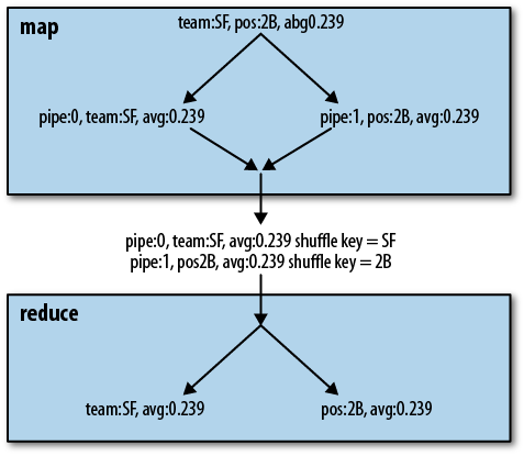
Pig can also combine multiple group
operators together in many cases. In the example given at the beginning of
this section, where the baseball data is grouped by both team and position, this
entire Pig Latin script will be executed inside one MapReduce job. Pig
accomplishes this by duplicating records on the map side and annotating
each record with its pipeline number. When the data is partitioned during
the shuffle, the appropriate key is used for each record. That is, records
from the pipeline grouping by team will
use team as their shuffle key, and
records from the pipeline grouping by position will use position as their shuffle key. This is done by
declaring the key type to be tuple and
placing the correct values in the key tuple for each record. Once the data
has been collected to reducers, the pipeline number is used as part of the
sort key so that records from each pipeline and group are collected
together. In the reduce task, Pig instantiates multiple pipelines, one for
each group operator. It sends each record down the appropriate pipeline
based on its annotated pipeline number. In this way, input data can be
scanned once but grouped many different ways. An example of how one record
flows through this pipeline is shown in Figure 6-1. Although this does not provide linear
speedup, we find it often approaches it.
There are cases where Pig will not combine
multiple operators into a single MapReduce job. Pig does not use
multiquery for any of the multiple-input operators: join, union, cross, or cogroup. It does not use multiquery for
order statements either. Also, if it has multiple
group statements and some would use Hadoop’s combiner and
some would not, it combines only those statements that use Hadoop’s
combiner into a multiquery. This is because we have found that combining
the Hadoop combiner and non-Hadoop combiner jobs together does not perform
well.
Multiquery scripts tend to perform better than
loading the same input multiple times, but this approach does have limits.
Because it requires replicating records in the map, it does slow down the
shuffle phase. Eventually the increased cost of the shuffle phase
outweighs the reduced cost of rescanning the input data. Pig has no way to
estimate when this will occur. Currently, the optimizer is optimistic and
always combines jobs with multiquery whenever it can. If it combines too
many jobs and becomes slower than splitting some of the jobs, you can turn
off multiquery or you can rewrite your Pig Latin into separate scripts so
Pig does not attempt to combine them all. To turn off multiquery, you can
pass either -M or -no_multiquery on the command line or set the
property opt.multiquery to false.
We must also consider what happens when one job in
a multiquery fails but others succeed. If all jobs succeed, Pig will
return 0, meaning success. If all of the jobs fail, Pig will return 2. If
some jobs fail and some succeed, Pig will return 3. By default, if one of
the jobs fails, Pig will continue processing the other jobs. However, if
you want Pig to stop as soon as one of the jobs fails, you can pass
-F or -stop_on_failure. In this case, any jobs that
have not yet been finished will be terminated, and any that have not
started will not be started. Any jobs that are already finished will not
be cleaned up.
In addition to providing many relational and dataflow operators, Pig Latin provides ways for you to control how your jobs execute on MapReduce. It allows you to set values that control your environment and details of MapReduce, such as how your data is partitioned.
The set command is used to set the
environment in which Pig runs the MapReduce jobs. Table 6-1 shows Pig-specific parameters that can be
controlled via set.
Table 6-1. Pig-specific set parameters
| Parameter | Value type | Description |
|---|---|---|
debug | string | Sets the logging level to DEBUG. Equivalent to passing -debug DEBUG on the command
line. |
default_parallel | integer | Sets a default parallel level for all reduce operations in the script. See Parallel for details. |
job.name | string | Assigns a name to the Hadoop job. By default the name is the filename of the script being run, or a randomly generated name for interactive sessions. |
job.priority | string | If your Hadoop cluster is using the Capacity Scheduler
with priorities enabled for queues, this allows you to set the
priority of your Pig job. Allowed values are very_low, low, normal, high, and very_high. |
For example, to set the default parallelism of
your Pig Latin script and set the job name to
my_job:
set default_parallel 10;
set job.name my_job;
users = load 'users';
In addition to these predefined values,
set can be used to pass Java property settings to Pig and Hadoop. Both Pig and
Hadoop use a number of Java properties to control their behavior.
Consider an example where you want to turn multiquery off for a given
script, and you want to tell Hadoop to use a higher value than usual for
its map-side sort buffer:
set opt.multiquery false;
set io.sort.mb 2048; --give it 2G
You can also use this mechanism to pass
properties to UDFs. All of the properties are passed to the tasks on the
Hadoop nodes when they are executed. They are not set as Java properties
in that environment; rather, they are placed in a Hadoop object called
JobConf. UDFs have access to the
JobConf. Thus, anything you set in the script can
be seen by your UDFs. This can be a convenient way to control UDF
behavior. For information on how to retrieve this information in your
UDFs, see Constructors and Passing Data from Frontend to Backend.
Values that are set in your script are global for the whole script. If they are reset later in the script, that second value will overwrite the first and be used throughout the whole script.
Hadoop uses a class called Partitioner to
partition records to reducers during the shuffle phase. For details on
partitioners, see Shuffle Phase. Pig does not
override the default partitioner, except for order and skew join. The balancing operations in these require
special Partitioners.
Beginning in version 0.8, Pig allows you to set
the partitioner, except in the cases where it is already overriding it.
To do this, you need to tell Pig which Java class to use to partition
your data. This class must extend Hadoop’s
org.apache.hadoop.mapreduce.Partitioner<KEY,VALUE>.
Note that this is the newer (version 0.20 and later) mapreduce API and not the older mapred:
register acme.jar; --jar containing the partitioner
users = load 'users' as (id, age, zip);
grp   = group users by id partition by com.acme.userpartitioner parallel 100;
Operators that reduce data can take the
partition clause. These operators are
cogroup, cross, distinct, group, and join (again, not in conjunction with skew
join).
Pig Latin has a preprocessor that runs before your Pig Latin
script is parsed. In 0.8 and earlier, this provided parameter substitution,
roughly similar to a very simple version of #define in C.
Starting with 0.9, it also provides inclusion of other Pig Latin scripts
and function-like macro definitions, so that you can write Pig Latin in a
modular way.
Pig Latin scripts that are used frequently often have elements that need to change based on when or where they are run. A script that is run every day is likely to have a date component in its input files or filters. Rather than edit and change the script every day, you want to pass in the date as a parameter. Parameter substitution provides this capability with a basic string-replacement functionality. Parameters must start with a letter or an underscore and can then have any amount of letters, numbers, or underscores. Values for the parameters can be passed in on the command line or from a parameter file:
--daily.pig
daily     = load 'NYSE_daily' as (exchange:chararray, symbol:chararray,
                date:chararray, open:float, high:float, low:float, close:float,
                volume:int, adj_close:float);
yesterday = filter daily by date == '$DATE';
grpd      = group yesterday all;
minmax    = foreach grpd generate MAX(yesterday.high), MIN(yesterday.low);
When you run daily.pig, you must provide a definition for
the parameter DATE; otherwise, you
will get an error telling you that you have undefined parameters:
pig -p DATE=2009-12-17 daily.pig
You can repeat the -p command-line switch as many times as
needed. Parameters can also be placed in a file, which is convenient if
you have more than a few of them. The format of the file is
parameter=value, one per line. Comments in
the file should be preceded by a #.
You then indicate the file to be used with -m or -param_file:
pig -param_file daily.params daily.pig
Parameters passed on the command line take precedence over parameters provided in files. This way, you can provide all your standard parameters in a file and override a few as needed on the command line.
Parameters can contain other parameters. So, for example, you could have the following parameter file:
#Param file
YEAR=2009-
MONTH=12-
DAY=17
DATE=$YEAR$MONTH$DAY
A parameter must be defined before it is
referenced. The parameter file here would produce an error if the
DAY line came after the DATE line. The other caveat is that there is
no special character to delimit the end of a parameter. Any alphanumeric
or underscore character will be interpreted as part of the parameter,
and any other character will be interpreted as itself. So, if you had a
script that ran at the first of every month, you could not do the
following:
wlogs = load 'clicks/$YEAR$MONTH01' as (url, pageid, timestamp);
This would try to resolve a parameter MONTH01 when you meant MONTH.
When using parameter substitution, all
parameters in your script must be resolved after the preprocessor is
finished. If not, Pig will issue an error message and not continue. You
can see the results of your parameter substitution by using the -dryrun flag on the Pig command line. Pig will
write out a version of your Pig Latin script with the parameter
substitution done, but it will not execute the script.
You can also define parameters inside your Pig
Latin script using %declare and %default. %declare allows
you to define a parameter in the script itself. %default is
useful to provide a common default value that can be overridden when
needed. Consider a case where most of the time your script is run on one
Hadoop cluster, but occasionally it is run on a different cluster with
different hardware:
%default parallel_factor 10;
wlogs = load 'clicks' as (url, pageid, timestamp);
grp   = group wlogs by pageid parallel $parallel_factor;
cntd  = foreach grp generate group, COUNT(wlogs);
When running your script in the usual
configuration, there is no need to set the parameter parallel_factor. On the occasions it is run in
a different setup, the parallel factor can be changed by passing a value
on the command line.
Starting in 0.9, Pig added the ability to define macros. This makes it possible to make your Pig Latin scripts modular. It also makes it possible to share segments of Pig Latin code among users. This can be particularly useful for defining standard practices and making sure all data producers and consumers use them.
Macros are declared with the define statement. A macro takes a set of
input parameters, which are string values that will be substituted for
the parameters when the macro is expanded. By convention, input relation
names are placed first before other parameters. The output relation name
is given in a returns statement. The operators of the macro
are enclosed in {} (braces). Anywhere
the parameters—including the output relation name—are referenced inside
the macro, they must be preceded by a $ (dollar sign). The
macro is then invoked in your Pig Latin by assigning it to a
relation:
--macro.pig
-- Given daily input and a particular year, analyze how
-- stock prices changed on days dividends were paid out.
define dividend_analysis (daily, year, daily_symbol, daily_open, daily_close)
returns analyzed {
    divs          = load 'NYSE_dividends' as (exchange:chararray,
                        symbol:chararray, date:chararray, dividends:float);
    divsthisyear  = filter divs by date matches '$year-.*';
    dailythisyear = filter $daily by date matches '$year-.*';
    jnd           = join divsthisyear by symbol, dailythisyear by $daily_symbol;
    $analyzed     = foreach jnd generate dailythisyear::$daily_symbol,
                        $daily_close - $daily_open;
};

daily   = load 'NYSE_daily' as (exchange:chararray, symbol:chararray,
            date:chararray, open:float, high:float, low:float, close:float,
            volume:int, adj_close:float);
results = dividend_analysis(daily, '2009', 'symbol', 'open', 'close');
It is also possible to have a macro that does
not return a relation. In this case, the returns clause of the define
statement is changed to returns void. This can be useful
when you want to define a macro that controls how data is partitioned
and sorted before being stored to a particular output, such as HBase or
a database.
These macros are expanded inline. This is where
an important difference between macros and functions becomes apparent.
Macros cannot be invoked recursively. Macros can invoke other macros, so
a macro A can invoke a macro B, but A
cannot invoke itself. And once A has
invoked B, B cannot invoke A. Pig will detect these loops and throw an
error.
Parameter substitution (see Parameter Substitution) cannot be used inside of macros. Parameters should be passed explicitly to macros, and parameter substitution should be used only at the top level.
You can use the -dryrun command-line
argument to see how the macros are expanded inline. When the macros are
expanded, the alias names are changed to avoid collisions with alias
names in the place the macro is being expanded. If we take the previous
example and use -dryrun to show us
the resulting Pig Latin, we will see the following (reformatted slightly
to fit on the page):
daily = load 'NYSE_daily' as (exchange:chararray, symbol:chararray,
            date:chararray, open:float, high:float, low:float, close:float,
            volume:int, adj_close:float);
macro_dividend_analysis_divs_0 = load 'NYSE_dividends' as (exchange:chararray,
            symbol:chararray, date:chararray, dividends:float);
macro_dividend_analysis_divsthisyear_0 =
            filter macro_dividend_analysis_divs_0 BY (date matches '2009-.*');
macro_dividend_analysis_dailythisyear_0 = filter daily BY (date matches '2009-.*');
macro_dividend_analysis_jnd_0 =
            join macro_dividend_analysis_divsthisyear_0 by (symbol),
            macro_dividend_analysis_dailythisyear_0 by (symbol);
results = foreach macro_dividend_analysis_jnd_0 generate
            macro_dividend_analysis_dailythisyear_0::symbol, close - open;
As you can see, the aliases in the macro are expanded with a combination of the macro name and the invocation number. This provides a unique key so that if other macros use the same aliases, or the same macro is used multiple times, there is still no duplication.
For a long time in Pig Latin, the entire script needed to be in one file. This produced some rather unpleasant multithousand-line Pig Latin scripts. Starting in 0.9, the preprocessor can be used to include one Pig Latin script in another. Taken together with the macros (also added in 0.9; see Macros), it is now possible to write modular Pig Latin that is easier to debug and reuse.
import is used to include one Pig Latin
script in another:
--main.pig
import '../examples/ch6/dividend_analysis.pig';

daily   = load 'NYSE_daily' as (exchange:chararray, symbol:chararray,
            date:chararray, open:float, high:float, low:float, close:float,
            volume:int, adj_close:float);
results = dividend_analysis(daily, '2009', 'symbol', 'open', 'close');
import writes the imported
file directly into your Pig Latin script in place of the
import statement. In the preceding example, the
contents of dividend_analysis.pig
will be placed immediately before the load statement. Note
that a file cannot be imported twice. If you wish to use the same
functionality multiple times, you should write it as a macro and import
the file with that macro.
In the example just shown, we used a relative
path for the file to be included. Fully qualified paths also can be
used. By default, relative paths are taken from the current working
directory of Pig when you launch the script. You can set a search path
by setting the pig.import.search.path property. This is a
comma-separated list of paths that will be searched for your files. The
current working directory, . (dot), is always in the search path:
set pig.import.search.path '/usr/local/pig,/grid/pig';
import 'acme/macros.pig';
Imported files are not in separate namespaces. This means that all macros are in the same namespace, even when they have been imported from separate files. Thus, care should be taken to choose unique names for your macros.
[15] Those with database experience will notice that this is a violation of the first normal form as defined by E. F. Codd. This intentional denormalization of data is very common in OLAP systems in general, and in large data-processing systems such as Hadoop in particular. RDBMS systems tend to make joins common and then work to optimize them. In systems such as Hadoop, where storage is cheap and joins are expensive, it is generally better to use nested data structures to avoid the joins.
[16] In versions 0.8 and earlier, there is a bug where
this flatten is assigned a schema of one field, which
is a bytearray, instead of causing the schema to be
null. This bug has been fixed in 0.9.
[17] This algorithm was proposed in the paper “Practical Skew Handling in Parallel Joins,” presented by David J. DeWitt, Jeffrey F. Naughton, Donovan A. Schneider, and S. Seshadri at the 18th International Conference on Very Large Databases.
[18] In 0.8 and earlier, the number of records is always 10. In 0.9, this is changed to be the square root of the parallel factor, rounded up.
Get Programming Pig now with the O’Reilly learning platform.
O’Reilly members experience books, live events, courses curated by job role, and more from O’Reilly and nearly 200 top publishers.

