Filter Ranges
Filters work by hiding rows that don’t meet certain criteria. Filter criteria are selected from drop-down lists in a column’s heading. You can select built-in criteria, such as Top 10, or enter your own custom criteria. To create a filter in Excel:
Select the header row of the rows you want to filter.
Choose Data → Filter → AutoFilter. Excel adds a filter drop-down list to each of the selected columns.
Tip
Lists provide a more powerful and flexible tool for filtering ranges . Lists are available only in Excel 2003, however.
To apply the filter, select the criteria from one of the drop-down lists as shown in Figure 11-2. Excel hides the rows below that don’t match the criteria. You can apply filters for more than one column to further narrow the range of displayed rows.
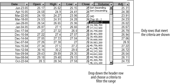
Figure 11-2. Applying a filter to a stock price history table
To create a filter in code, use the Range object’s AutoFilter method without arguments. To apply a filter, call AutoFilter again with the column to filter and the criteria as arguments. The following ApplyFilter procedure creates a filter and applies a filter to display 10 days with the most volume (column 6 in Figure 11-2):
Sub ApplyFilter(  )
    Dim header As Range
    Set header = [e21:k21]
    ' Create filter
    header.AutoFilter
    ' Apply filter to show top 10 volume days.
    header.AutoFilter 6, "10", XlAutoFilterOperator.xlTop10Items
End Sub
Tip
You’ve got ...
Get Programming Excel with VBA and .NET now with the O’Reilly learning platform.
O’Reilly members experience books, live events, courses curated by job role, and more from O’Reilly and nearly 200 top publishers.

