11
Model Conversion from Discrete-Time to Continuous-Time Linear Models
11.1 Transfer Function of Discrete-Time Processes
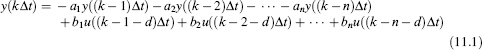
In Part One, the Laplace transform was used to derive the transfer function of a continuous-time process. For a discrete-time process, the z-tranform is used. Consider the following discrete-time process:
The z-transform of y(kΔt) is defined as
![]()
One of the notable properties of the z-transform is y(z)z−1 = Z{y(k − 1)Δt)} if y(kΔt) = 0, k < 0. The property is derived straightforwardly by comparing (11.2) with (11.3):
![]()
From (11.2) and (11.3), it is clear that y(z)z−1 = Z{y(k − 1)Δt)} if y(kΔt) = 0, k < 0. Equivalently, y(z)z−d = Z{y(k − d)Δt)} if y(kΔt) = 0, k < 0. Then, (11.4) is obtained by applying the z-transform to (11.1):
![]()
Rearranging (11.4), the following transfer function for the discrete-time process is obtained:
![]()
or
![]()
11.2 Frequency Responses of Discrete-Time Processes ...
Get Process Identification and PID Control now with the O’Reilly learning platform.
O’Reilly members experience books, live events, courses curated by job role, and more from O’Reilly and nearly 200 top publishers.

