
187
14
Frequency Modelling: Selecting and
Calibrating a Frequency Model
The objective of frequency modelling is the production of a model that gives you the prob-
ability of a given number of losses occurring during a given period, such as the policy
period or a calendar year. As is the case with all models we use for pricing, the frequency
model may be based to a varying extent on past losses, but it is a prospective model, that
is, it tells you what the number of losses will be in the future. As such, loss experience will
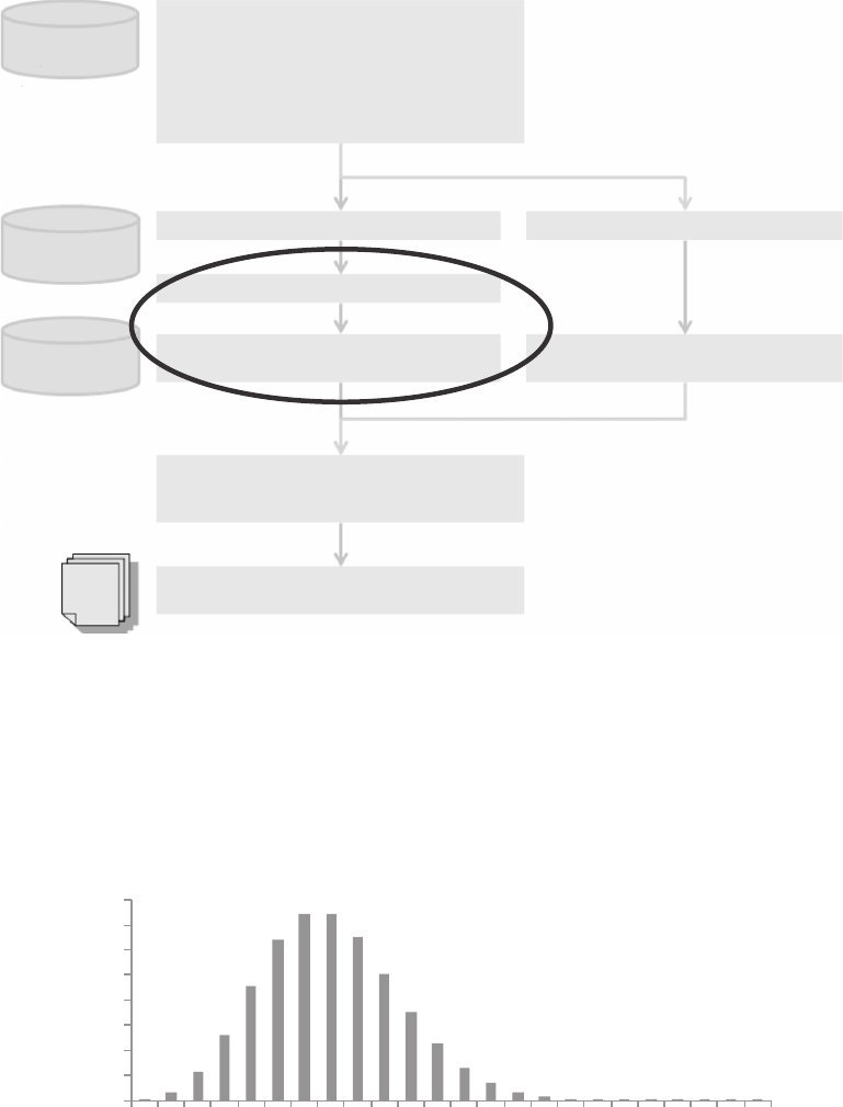
have to be adapted to current circumstances before it can be used (Figure 14.1).
Figure 14.2 gives an example of how a frequency model (in this case a Poisson model
with an average frequency of 7) might look like: as an example, it tells us that the probabil-
ity of having exactly four claims is approximately 0.091, and that the probability of having
up to four claims is approximately 0.173.
Theoretically, there are innitely many models that one could use for frequency. In prac-
tice, however, because there are only a small number of years/periods of experience that
one can use to t a frequency model (typically 5–10 years, but it can be as small as 1 year) it
is not possible to discriminate between many models, and in the spirit of statistical learn-
ing (see Section 12.3), it is better to rely on a few well-tested models that one can trust and
that are analytically tractable and choose from among them rather than having a large
dictionary of models that one can choose from on the basis of imsy statistical evidence.
The three most popular models used in insurance are probably the binomial distribution, the
Poisson distribution and the negative binomial distribution. All three of them are so-called ‘count-
ing distributions’, that is, discrete distributions with values over the natural numbers only.
The main practical difference between these three models is that they have different
variance/mean ratios: this is 1 for the Poisson distribution, less than 1 for the binomial
distribution and greater than 1 for the negative binomial distribution. A calculation of the
variance/mean ratio of the number of claims over a certain period may therefore be the
factor that drives the choice of what model is used, although, as we will soon show, things
are more complicated than that.
In practice, the binomial distribution (and its relative, the multinomial distribution) is
normally used with the individual risk model, whereas the Poisson and negative binomial
are used with the collective risk model.
Not only are these three models very simple but they also have some useful properties:
all of them are part of the Panjer class, and they are the only distributions belonging to this
class. The Panjer class (also referred to as the [a,b,0] class) is characterised by the fact that
there exist constants a and b such that
p
p
a
b
k
k
k
k−
=+
=…
1
123
,,
, (14.1)
where p
k
is the probability of having exactly k losses, and p
0
is uniquely determined by
imposing the condition
p
k
k
=
=
∞
∑
1
0
.
188 Pricing in General Insurance
Individual
loss data
Assumptions on
– Loss inflation
– Cu
rrency conversion
– …
Exposure
data
Portfolio/market
information
Data preparation
– Data checking
– Data cleansing
– Data transformation
– Claims revaluation and currency conversion
– Data summarisation
– Calculation of simple statistics
Inputs to frequency/severity analysis
Adjust historical claim counts for IBNR
Adjust for exposure/profile changes
le
Select frequency distribution and
calibrate parameters
Adjust loss amounts for IBNER
Severity model
Frequency model
Estimate gross aggregate distribution
e.g. Monte Carlo simulation, Fast Fourier
transform, Panjer recursion…
Gross aggregate loss model
Ceded/retained aggregate loss model
Allocate losses between (re)insurer and
(re)insured
Cover
data
Se ct severity distribution and
calibrate parameters
FIGURE 14.1
How selecting and calibrating a frequency model ts in the risk costing subprocess.
0
0.02
0.04
0.06
0.08
0.1
0.12
0.14
0.16
012345678910 11 12 13 14 15 16 17 18 19 20 21 22
No. of claims
Probability
Frequency Model - An Example
Poisson with Rate = 7
FIGURE 14.2
An example of a frequency distribution – a Poisson distribution with rate = 7. The distribution is obviously
asymmetrical – only numbers greater than or equal to 0 have a probability greater than 0, whereas the distribu-
tion extends indenitely to the right.
Get Pricing in General Insurance now with the O’Reilly learning platform.
O’Reilly members experience books, live events, courses curated by job role, and more from O’Reilly and nearly 200 top publishers.

