Chapter 4
Solving a System of Linear Equations
Core Topics
Gauss elimination method (4.2).
Gauss elimination with pivoting (4.3).
Gauss–Jordan elimination method (4.4).
LU decomposition method (4.5).
Inverse of a matrix (4.6)
Iterative methods (Jacobi, Gauss–Seidel) (4.7).
Use of MATLAB's built-in functions for solving a system of linear equations (4.8).
Complementary Topics
Tridiagonal systems of equations (4.9).
Error, residual, norms, and condition number (4.10).
Ill-conditioned systems (4.11).
4.1 BACKGROUND
Systems of linear equations that have to be solved simultaneously arise in problems that include several (possibly many) variables that are dependent on each other. Such problems occur not only in engineering and science, which are the focus of this book, but in virtually any discipline (business, statistics, economics, etc.). A system of two (or three) equations with two (or three) unknowns can be solved manually by substitution or other mathematical methods (e.g., Cramer's rule, Section 2.4.6). Solving a system in this way is practically impossible as the number of equations (and unknowns) increases beyond three.
An example of a problem in electrical engineering that requires a solution of a system of equations is shown in Fig. 4-1. Using Kirchhoff's law, the currents i1, i2, i3, and i4 can be determined by solving the following system of four equations:
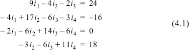
Figure 4-1: ...
Get Numerical Methods for Engineers and Scientists 3rd Edition now with the O’Reilly learning platform.
O’Reilly members experience books, live events, courses curated by job role, and more from O’Reilly and nearly 200 top publishers.

