Next Generation Excel: Modeling In Excel For Analysts And MBAs (For MS Windows And Mac OS), 2nd Edition

Chapter 28

Using Slicers to Filter Pivot Tables

The new versions of Excel 2010 incorporate special button-style filters named Slicers. This new tool makes it possible to filter Pivot Table data while indicating the filtering state of the data/filter, thus enabling you to understand and visualize which data is part of the report while you view it.

In a way the Slicer is also like a Scenario Manager—when you filter certain data you see its impact on the PivotTable data. This is a way to understand Pivot Tables better. Adding the Slicer makes it much easier to manipulate the data.

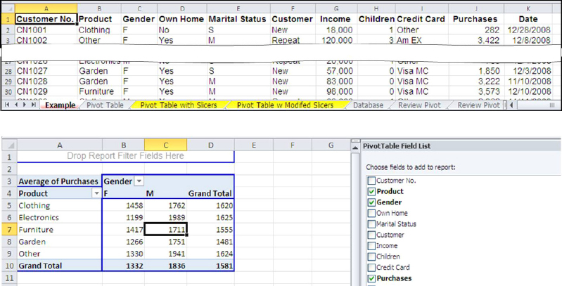
Refer back to the data we used in Chapter 27 on the sheet Example. The sheet Pivot Table has an example of a PivotTable created from the data on the sheet Example. See Figure 28.1.

FIGURE 28.1 The Data of the Example Sheet and the Pivot Table

Using conventional Pivot Table filters does not have the same effect as the Slicer does. Follow these steps to create a Slicer for the above example.

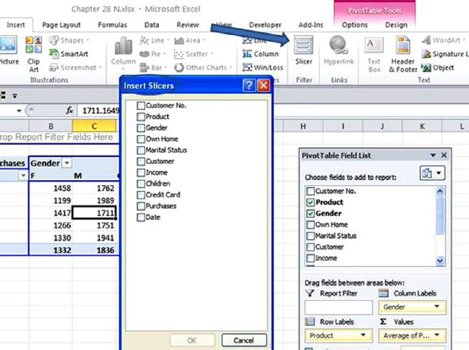
To activate Slicer, click on the Slicer icon under the Insert Ribbon. The Insert Slicer menu will appear. You can choose any or as many of the parameters/headers, you would like to use for filtering the data. In this example, I selected Own Home and Children. See Figure 28.2.

FIGURE 28.2 Activating the Slicer

Figure ...