Chapter 5
Conditional and Advanced Conditional Formatting in Excel
Conditional formatting is just what it says: formatting a cell based on its contents, usually a value. You may want to have a specific color or font type for a specific range of values. Conditional Formatting used to have, in older versions of Excel, up to three format conditions in addition to the default “no format” condition. Starting in Excel 2007 you may use many other features of conditional formatting. This chapter explains most of these features.
When using the old versions Excel, all you had to do is go through the menu to Format=>Conditional Formatting and apply the rules. As mentioned above, you could have up to three formats in a single cell or range of cells.
With the newer versions, starting in Excel 2007, conditional formatting became more comprehensive and allows you to be more creative.
SIMPLE CONDITIONAL FORMATTING; ADDING A RULE
The simplest way to apply a single rule is to select Conditional Formatting under the home Ribbon. Click on “Highlight Cells Rules” and choose one of the rules on the left. Excel has seven rules you may choose from. You also have a choice to create your own personalized rules. See Figure 5.1.
FIGURE 5.1 Choose a Conditional Formatting Rule
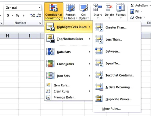
These rule choices are simpler to manipulate than in older versions of Excel. Now you can indicate with two clicks the format a cell ...
Get Next Generation Excel: Modeling In Excel For Analysts And MBAs (For MS Windows And Mac OS), 2nd Edition now with the O’Reilly learning platform.
O’Reilly members experience books, live events, courses curated by job role, and more from O’Reilly and nearly 200 top publishers.

