Let’s return to our exploration of the ways we can bring our computational resources to bear on large quantities of text. We began this discussion in Computing with Language: Texts and Words, and saw how to search for words in context, how to compile the vocabulary of a text, how to generate random text in the same style, and so on.
In this section, we pick up the question of what makes a text distinct, and use automatic methods to find characteristic words and expressions of a text. As in Computing with Language: Texts and Words, you can try new features of the Python language by copying them into the interpreter, and you’ll learn about these features systematically in the following section.
Before continuing further, you might like to check your understanding of the last section by predicting the output of the following code. You can use the interpreter to check whether you got it right. If you’re not sure how to do this task, it would be a good idea to review the previous section before continuing further.
>>> saying = ['After', 'all', 'is', 'said', 'and', 'done',
...           'more', 'is', 'said', 'than', 'done']
>>> tokens = set(saying)
>>> tokens = sorted(tokens)
>>> tokens[-2:]
what output do you expect here?
>>>
How can we automatically identify the words of a text that are most informative about the topic and genre of the text? Imagine how you might go about finding the 50 most frequent words of a book. One method would be to keep a tally for each vocabulary item, like that shown in Figure 1-3. The tally would need thousands of rows, and it would be an exceedingly laborious process—so laborious that we would rather assign the task to a machine.
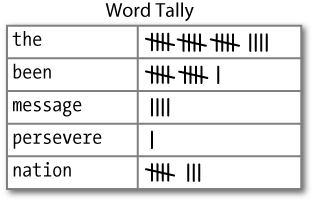
The table in Figure 1-3 is known as a
frequency distribution , and it tells us the frequency of each vocabulary item
in the text. (In general, it could count any kind of observable
event.) It is a “distribution” since it tells us how the total number
of word tokens in the text are distributed across the vocabulary
items. Since we often need frequency distributions in language
processing, NLTK provides built-in support for them. Let’s use a
FreqDist to find the 50 most frequent words of Moby
Dick. Try to work out what is going on here, then read the
explanation that follows.
>>> fdist1 = FreqDist(text1)>>> fdist1
<FreqDist with 260819 outcomes> >>> vocabulary1 = fdist1.keys()
>>> vocabulary1[:50]
[',', 'the', '.', 'of', 'and', 'a', 'to', ';', 'in', 'that', "'", '-', 'his', 'it', 'I', 's', 'is', 'he', 'with', 'was', 'as', '"', 'all', 'for', 'this', '!', 'at', 'by', 'but', 'not', '--', 'him', 'from', 'be', 'on', 'so', 'whale', 'one', 'you', 'had', 'have', 'there', 'But', 'or', 'were', 'now', 'which', '?', 'me', 'like'] >>> fdist1['whale'] 906 >>>
When we first invoke FreqDist, we pass the name of the text as an argument ![]() . We can inspect the total number of
words (“outcomes”) that have been counted up
. We can inspect the total number of
words (“outcomes”) that have been counted up ![]() —260,819 in the case of
Moby Dick. The expression
—260,819 in the case of
Moby Dick. The expression keys() gives us a list of all the distinct types in the text
![]() , and we can look at the first 50
of these by slicing the list
, and we can look at the first 50
of these by slicing the list ![]() .
.
Note
Your Turn: Try the
preceding frequency distribution example for yourself, for text2. Be careful to use the correct
parentheses and uppercase letters. If you get an error message
NameError: name 'FreqDist' is not
          defined
, you need to start your work with from nltk.book import *.
Do any words produced in the last example help us grasp the
topic or genre of this text? Only one word,
whale, is slightly informative! It occurs over
900 times. The rest of the words tell us nothing about the text;
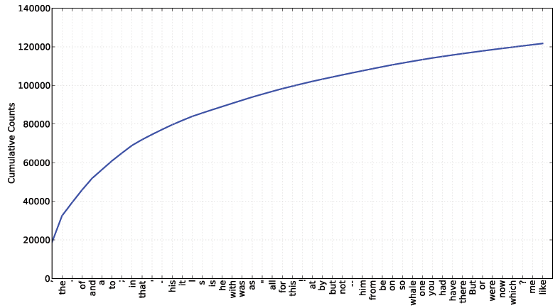
they’re just English “plumbing.” What proportion of the text is taken
up with such words? We can generate a cumulative frequency plot for
these words, using fdist1.plot(50,
cumulative=True), to produce the graph in Figure 1-4. These 50 words account for nearly half
the book!
If the frequent words don’t help us, how about the words that
occur once only, the so-called hapaxes? View them by typing fdist1.hapaxes(). This list contains
lexicographer,
cetological, contraband,
expostulations, and about 9,000 others. It seems
that there are too many rare words, and without seeing the context we
probably can’t guess what half of the hapaxes mean in any case! Since
neither frequent nor infrequent words help, we need to try something
else.
Next, let’s look at the long words of a text; perhaps these will be more characteristic and informative. For this we adapt some notation from set theory. We would like to find the words from the vocabulary of the text that are more than 15 characters long. Let’s call this property P, so that P(w) is true if and only if w is more than 15 characters long. Now we can express the words of interest using mathematical set notation as shown in a. This means “the set of all w such that w is an element of V (the vocabulary) and w has property P.”
The corresponding Python expression is given in b. (Note that it produces a list, not a set, which means that duplicates are possible.) Observe how similar the two notations are. Let’s go one more step and write executable Python code:
>>> V = set(text1)
>>> long_words = [w for w in V if len(w) > 15]
>>> sorted(long_words)
['CIRCUMNAVIGATION', 'Physiognomically', 'apprehensiveness', 'cannibalistically',
'characteristically', 'circumnavigating', 'circumnavigation', 'circumnavigations',
'comprehensiveness', 'hermaphroditical', 'indiscriminately', 'indispensableness',
'irresistibleness', 'physiognomically', 'preternaturalness', 'responsibilities',
'simultaneousness', 'subterraneousness', 'supernaturalness', 'superstitiousness',
'uncomfortableness', 'uncompromisedness', 'undiscriminating', 'uninterpenetratingly']
>>>
For each word w in the
vocabulary V, we check whether
len(w) is greater than 15; all
other words will be ignored. We will discuss this syntax more
carefully later.
Note
Your Turn: Try out the
previous statements in the Python interpreter, and experiment with
changing the text and changing the length condition. Does it make an
difference to your results if you change the variable names, e.g.,
using [word for word in vocab if
...]?
Let’s return to our task of finding words that characterize a
text. Notice that the long words in text4 reflect its national
focus—constitutionally,
transcontinental—whereas those in text5 reflect its informal content:
boooooooooooglyyyyyy and
yuuuuuuuuuuuummmmmmmmmmmm. Have we succeeded in
automatically extracting words that typify a text? Well, these very
long words are often hapaxes (i.e., unique) and perhaps it would be
better to find frequently occurring long words.
This seems promising since it eliminates frequent short words (e.g.,
the) and infrequent long words (e.g.,
antiphilosophists). Here are all words from the
chat corpus that are longer than seven characters, that occur more
than seven times:
>>> fdist5 = FreqDist(text5)
>>> sorted([w for w in set(text5) if len(w) > 7 and fdist5[w] > 7])
['#14-19teens', '#talkcity_adults', '((((((((((', '........', 'Question',
'actually', 'anything', 'computer', 'cute.-ass', 'everyone', 'football',
'innocent', 'listening', 'remember', 'seriously', 'something', 'together',
'tomorrow', 'watching']
>>>
Notice how we have used two conditions: len(w) > 7 ensures that the words are
longer than seven letters, and fdist5[w] >
7 ensures that these words occur more than seven times. At
last we have managed to automatically identify the frequently
occurring content-bearing words of the text. It is a modest but
important milestone: a tiny piece of code, processing tens of
thousands of words, produces some informative output.
A collocation is a sequence of words that occur together unusually often. Thus red wine is a collocation, whereas the wine is not. A characteristic of collocations is that they are resistant to substitution with words that have similar senses; for example, maroon wine sounds very odd.
To get a handle on collocations, we start off by extracting from
a text a list of word pairs, also known as bigrams. This is easily accomplished with the
function bigrams():
>>> bigrams(['more', 'is', 'said', 'than', 'done'])
[('more', 'is'), ('is', 'said'), ('said', 'than'), ('than', 'done')]
>>>
Here we see that the pair of words
than-done is a bigram, and we write it in Python
as ('than', 'done'). Now,
collocations are essentially just frequent bigrams, except that we
want to pay more attention to the cases that involve rare words. In
particular, we want to find bigrams that occur more often than we
would expect based on the frequency of individual words. The collocations() function does this for us (we will see how it works
later):
>>> text4.collocations()
Building collocations list
United States; fellow citizens; years ago; Federal Government; General
Government; American people; Vice President; Almighty God; Fellow
citizens; Chief Magistrate; Chief Justice; God bless; Indian tribes;
public debt; foreign nations; political parties; State governments;
National Government; United Nations; public money
>>> text8.collocations()
Building collocations list
medium build; social drinker; quiet nights; long term; age open;
financially secure; fun times; similar interests; Age open; poss
rship; single mum; permanent relationship; slim build; seeks lady;
Late 30s; Photo pls; Vibrant personality; European background; ASIAN
LADY; country drives
>>>
The collocations that emerge are very specific to the genre of the texts. In order to find red wine as a collocation, we would need to process a much larger body of text.
Counting words is useful, but we can count other things too. For
example, we can look at the distribution of word lengths in a text, by
creating a FreqDist out of a long list of numbers, where each number is the
length of the corresponding word in the text:
>>> [len(w) for w in text1]
We start by deriving a list of the lengths of words in text1 ![]() ,
and the
,
and the FreqDist then counts the number of times each of these occurs
![]() . The result
. The result ![]() is a distribution containing a
quarter of a million items, each of which is a number corresponding to
a word token in the text. But there are only 20 distinct items being
counted, the numbers 1 through 20, because there are only 20 different
word lengths. I.e., there are words consisting of just 1 character, 2
characters, ..., 20 characters, but none with 21 or more characters.
One might wonder how frequent the different lengths of words are
(e.g., how many words of length 4 appear in the text, are there more
words of length 5 than length 4, etc.). We can do this as
follows:
is a distribution containing a
quarter of a million items, each of which is a number corresponding to
a word token in the text. But there are only 20 distinct items being
counted, the numbers 1 through 20, because there are only 20 different
word lengths. I.e., there are words consisting of just 1 character, 2
characters, ..., 20 characters, but none with 21 or more characters.
One might wonder how frequent the different lengths of words are
(e.g., how many words of length 4 appear in the text, are there more
words of length 5 than length 4, etc.). We can do this as
follows:
>>> fdist.items()
[(3, 50223), (1, 47933), (4, 42345), (2, 38513), (5, 26597), (6, 17111), (7, 14399),
(8, 9966), (9, 6428), (10, 3528), (11, 1873), (12, 1053), (13, 567), (14, 177),
(15, 70), (16, 22), (17, 12), (18, 1), (20, 1)]
>>> fdist.max()
3
>>> fdist[3]
50223
>>> fdist.freq(3)
0.19255882431878046
>>>
From this we see that the most frequent word length is 3, and that words of length 3 account for roughly 50,000 (or 20%) of the words making up the book. Although we will not pursue it here, further analysis of word length might help us understand differences between authors, genres, or languages. Table 1-2 summarizes the functions defined in frequency distributions.
Table 1-2. Functions defined for NLTK’s frequency distributions
Example | Description |
|---|---|
Create a frequency distribution containing the given samples | |
| Increment the count for this sample |
| Count of the number of times a given sample occurred |
| Frequency of a given sample |
| Total number of samples |
| The samples sorted in order of decreasing frequency |
| Iterate over the samples, in order of decreasing frequency |
| Sample with the greatest count |
| Tabulate the frequency distribution |
| Graphical plot of the frequency distribution |
| Cumulative plot of the frequency distribution |
| Test if samples in |
Our discussion of frequency distributions has introduced some important Python concepts, and we will look at them systematically in Back to Python: Making Decisions and Taking Control.
Get Natural Language Processing with Python now with the O’Reilly learning platform.
O’Reilly members experience books, live events, courses curated by job role, and more from O’Reilly and nearly 200 top publishers.

