Natural Language Processing with Python

Chapter 1. Language Processing and Python

It is easy to get our hands on millions of words of text. What can we do with it, assuming we can write some simple programs? In this chapter, we’ll address the following questions:

1. What can we achieve by combining simple programming techniques with large quantities of text?

2. How can we automatically extract key words and phrases that sum up the style and content of a text?

3. What tools and techniques does the Python programming language provide for such work?

4. What are some of the interesting challenges of natural language processing?

This chapter is divided into sections that skip between two quite different styles. In the “computing with language” sections, we will take on some linguistically motivated programming tasks without necessarily explaining how they work. In the “closer look at Python” sections we will systematically review key programming concepts. We’ll flag the two styles in the section titles, but later chapters will mix both styles without being so up-front about it. We hope this style of introduction gives you an authentic taste of what will come later, while covering a range of elementary concepts in linguistics and computer science. If you have basic familiarity with both areas, you can skip to Automatic Natural Language Understanding; we will repeat any important points in later chapters, and if you miss anything you can easily consult the online reference material at http://www.nltk.org/. If the material is completely new to you, this chapter will raise more questions than it answers, questions that are addressed in the rest of this book.

Computing with Language: Texts and Words

We’re all very familiar with text, since we read and write it every day. Here we will treat text as raw data for the programs we write, programs that manipulate and analyze it in a variety of interesting ways. But before we can do this, we have to get started with the Python interpreter.

Getting Started with Python

One of the friendly things about Python is that it allows you to type directly into the interactive interpreter—the program that will be running your Python programs. You can access the Python interpreter using a simple graphical interface called the Interactive DeveLopment Environment (IDLE). On a Mac you can find this under Applications→MacPython, and on Windows under All Programs→Python. Under Unix you can run Python from the shell by typing idle (if this is not installed, try typing python). The interpreter will print a blurb about your Python version; simply check that you are running Python 2.4 or 2.5 (here it is 2.5.1):

Python 2.5.1 (r251:54863, Apr 15 2008, 22:57:26)
[GCC 4.0.1 (Apple Inc. build 5465)] on darwin
Type "help", "copyright", "credits" or "license" for more information.
>>>

Note

If you are unable to run the Python interpreter, you probably don’t have Python installed correctly. Please visit http://python.org/ for detailed instructions.

The >>> prompt indicates that the Python interpreter is now waiting for input. When copying examples from this book, don’t type the “>>>” yourself. Now, let’s begin by using Python as a calculator:

>>> 1 + 5 * 2 - 3
8
>>>

Once the interpreter has finished calculating the answer and displaying it, the prompt reappears. This means the Python interpreter is waiting for another instruction.

Note

Your Turn: Enter a few more expressions of your own. You can use asterisk (*) for multiplication and slash (/) for division, and parentheses for bracketing expressions. Note that division doesn’t always behave as you might expect—it does integer division (with rounding of fractions downwards) when you type 1/3 and “floating-point” (or decimal) division when you type 1.0/3.0. In order to get the expected behavior of division (standard in Python 3.0), you need to type: from __future__ import division.

The preceding examples demonstrate how you can work interactively with the Python interpreter, experimenting with various expressions in the language to see what they do. Now let’s try a non-sensical expression to see how the interpreter handles it:

>>> 1 +
  File "<stdin>", line 1
    1 +
      ^
SyntaxError: invalid syntax
>>>

This produced a syntax error. In Python, it doesn’t make sense to end an instruction with a plus sign. The Python interpreter indicates the line where the problem occurred (line 1 of <stdin>, which stands for “standard input”).

Now that we can use the Python interpreter, we’re ready to start working with language data.

Getting Started with NLTK

Before going further you should install NLTK, downloadable for free from http://www.nltk.org/. Follow the instructions there to download the version required for your platform.

Once you’ve installed NLTK, start up the Python interpreter as before, and install the data required for the book by typing the following two commands at the Python prompt, then selecting the book collection as shown in Figure 1-1.

>>> import nltk
>>> nltk.download()

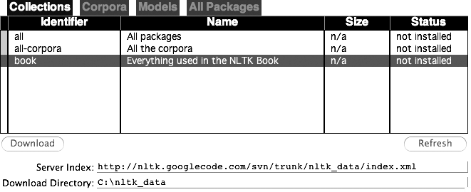
Figure 1-1. Downloading the NLTK Book Collection: Browse the available packages using nltk.download(). The Collections tab on the downloader shows how the packages are grouped into sets, and you should select the line labeled book to obtain all data required for the examples and exercises in this book. It consists of about 30 compressed files requiring about 100Mb disk space. The full collection of data (i.e., all in the downloader) is about five times this size (at the time of writing) and continues to expand.

Once the data is downloaded to your machine, you can load some of it using the Python interpreter. The first step is to type a special command at the Python prompt, which tells the interpreter to load some texts for us to explore: from nltk.book import *. This says “from NLTK’s book module, load all items.” The book module contains all the data you will need as you read this chapter. After printing a welcome message, it loads the text of several books (this will take a few seconds). Here’s the command again, together with the output that you will see. Take care to get spelling and punctuation right, and remember that you don’t type the >>>.

>>> from nltk.book import *
*** Introductory Examples for the NLTK Book ***
Loading text1, ..., text9 and sent1, ..., sent9
Type the name of the text or sentence to view it.
Type: 'texts()' or 'sents()' to list the materials.
text1: Moby Dick by Herman Melville 1851
text2: Sense and Sensibility by Jane Austen 1811
text3: The Book of Genesis
text4: Inaugural Address Corpus
text5: Chat Corpus
text6: Monty Python and the Holy Grail
text7: Wall Street Journal
text8: Personals Corpus
text9: The Man Who Was Thursday by G . K . Chesterton 1908
>>>

Any time we want to find out about these texts, we just have to enter their names at the Python prompt:

>>> text1
<Text: Moby Dick by Herman Melville 1851>
>>> text2
<Text: Sense and Sensibility by Jane Austen 1811>
>>>

Now that we can use the Python interpreter, and have some data to work with, we’re ready to get started.

Searching Text

There are many ways to examine the context of a text apart from simply reading it. A concordance view shows us every occurrence of a given word, together with some context. Here we look up the word monstrous in Moby Dick by entering text1 followed by a period, then the term concordance, and then placing "monstrous" in parentheses:

>>> text1.concordance("monstrous")
Building index...
Displaying 11 of 11 matches:
ong the former , one was of a most monstrous size . ... This came towards us ,
ON OF THE PSALMS . " Touching that monstrous bulk of the whale or ork we have r
ll over with a heathenish array of monstrous clubs and spears . Some were thick
d as you gazed , and wondered what monstrous cannibal and savage could ever hav
that has survived the flood ; most monstrous and most mountainous ! That Himmal
they might scout at Moby Dick as a monstrous fable , or still worse and more de
th of Radney .'" CHAPTER 55 Of the monstrous Pictures of Whales . I shall ere l
ing Scenes . In connexion with the monstrous pictures of whales , I am strongly
ere to enter upon those still more monstrous stories of them which are to be fo
ght have been rummaged out of this monstrous cabinet there is no telling . But
of Whale - Bones ; for Whales of a monstrous size are oftentimes cast up dead u
>>>

Note

Your Turn: Try searching for other words; to save re-typing, you might be able to use up-arrow, Ctrl-up-arrow, or Alt-p to access the previous command and modify the word being searched. You can also try searches on some of the other texts we have included. For example, search Sense and Sensibility for the word affection, using text2.concordance("affection"). Search the book of Genesis to find out how long some people lived, using: text3.concordance("lived"). You could look at text4, the Inaugural Address Corpus, to see examples of English going back to 1789, and search for words like nation, terror, god to see how these words have been used differently over time. We’ve also included text5, the NPS Chat Corpus: search this for unconventional words like im, ur, lol. (Note that this corpus is uncensored!)

Once you’ve spent a little while examining these texts, we hope you have a new sense of the richness and diversity of language. In the next chapter you will learn how to access a broader range of text, including text in languages other than English.

A concordance permits us to see words in context. For example, we saw that monstrous occurred in contexts such as the ___ pictures and the ___ size. What other words appear in a similar range of contexts? We can find out by appending the term similar to the name of the text in question, then inserting the relevant word in parentheses:

>>> text1.similar("monstrous")
Building word-context index...
subtly impalpable pitiable curious imperial perilous trustworthy
abundant untoward singular lamentable few maddens horrible loving lazy
mystifying christian exasperate puzzled
>>> text2.similar("monstrous")
Building word-context index...
very exceedingly so heartily a great good amazingly as sweet
remarkably extremely vast
>>>

Observe that we get different results for different texts. Austen uses this word quite differently from Melville; for her, monstrous has positive connotations, and sometimes functions as an intensifier like the word very.

The term common_contexts allows us to examine just the contexts that are shared by two or more words, such as monstrous and very. We have to enclose these words by square brackets as well as parentheses, and separate them with a comma:

>>> text2.common_contexts(["monstrous", "very"])
be_glad am_glad a_pretty is_pretty a_lucky
>>>

Note

Your Turn: Pick another pair of words and compare their usage in two different texts, using the similar() and common_contexts() functions.

It is one thing to automatically detect that a particular word occurs in a text, and to display some words that appear in the same context. However, we can also determine the location of a word in the text: how many words from the beginning it appears. This positional information can be displayed using a dispersion plot. Each stripe represents an instance of a word, and each row represents the entire text. In Figure 1-2 we see some striking patterns of word usage over the last 220 years (in an artificial text constructed by joining the texts of the Inaugural Address Corpus end-to-end). You can produce this plot as shown below. You might like to try more words (e.g., liberty, constitution) and different texts. Can you predict the dispersion of a word before you view it? As before, take care to get the quotes, commas, brackets, and parentheses exactly right.

>>> text4.dispersion_plot(["citizens", "democracy", "freedom", "duties", "America"])
>>>

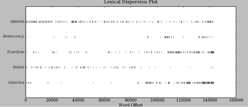
Figure 1-2. Lexical dispersion plot for words in U.S. Presidential Inaugural Addresses: This can be used to investigate changes in language use over time.

Note

Important: You need to have Python’s NumPy and Matplotlib packages installed in order to produce the graphical plots used in this book. Please see http://www.nltk.org/ for installation instructions.

Now, just for fun, let’s try generating some random text in the various styles we have just seen. To do this, we type the name of the text followed by the term generate. (We need to include the parentheses, but there’s nothing that goes between them.)

>>> text3.generate()
In the beginning of his brother is a hairy man , whose top may reach
unto heaven ; and ye shall sow the land of Egypt there was no bread in
all that he was taken out of the month , upon the earth . So shall thy
wages be ? And they made their father ; and Isaac was old , and kissed
him : and Laban with his cattle in the midst of the hands of Esau thy
first born , and Phichol the chief butler unto his son Isaac , she
>>>

Note that the first time you run this command, it is slow because it gathers statistics about word sequences. Each time you run it, you will get different output text. Now try generating random text in the style of an inaugural address or an Internet chat room. Although the text is random, it reuses common words and phrases from the source text and gives us a sense of its style and content. (What is lacking in this randomly generated text?)

Note

When generate produces its output, punctuation is split off from the preceding word. While this is not correct formatting for English text, we do it to make clear that words and punctuation are independent of one another. You will learn more about this in Chapter 3.

Counting Vocabulary

The most obvious fact about texts that emerges from the preceding examples is that they differ in the vocabulary they use. In this section, we will see how to use the computer to count the words in a text in a variety of useful ways. As before, you will jump right in and experiment with the Python interpreter, even though you may not have studied Python systematically yet. Test your understanding by modifying the examples, and trying the exercises at the end of the chapter.

Let’s begin by finding out the length of a text from start to finish, in terms of the words and punctuation symbols that appear. We use the term len to get the length of something, which we’ll apply here to the book of Genesis:

>>> len(text3)
44764
>>>

So Genesis has 44,764 words and punctuation symbols, or “tokens.” A token is the technical name for a sequence of characters—such as hairy, his, or :)—that we want to treat as a group. When we count the number of tokens in a text, say, the phrase to be or not to be, we are counting occurrences of these sequences. Thus, in our example phrase there are two occurrences of to, two of be, and one each of or and not. But there are only four distinct vocabulary items in this phrase. How many distinct words does the book of Genesis contain? To work this out in Python, we have to pose the question slightly differently. The vocabulary of a text is just the set of tokens that it uses, since in a set, all duplicates are collapsed together. In Python we can obtain the vocabulary items of text3 with the command: set(text3). When you do this, many screens of words will fly past. Now try the following:

>>> sorted(set(text3)) 
['!', "'", '(', ')', ',', ',)', '.', '.)', ':', ';', ';)', '?', '?)',
'A', 'Abel', 'Abelmizraim', 'Abidah', 'Abide', 'Abimael', 'Abimelech',
'Abr', 'Abrah', 'Abraham', 'Abram', 'Accad', 'Achbor', 'Adah', ...]
>>> len(set(text3)) 
2789
>>>

By wrapping sorted() around the Python expression set(text3) , we obtain a sorted list of vocabulary items, beginning with various punctuation symbols and continuing with words starting with A. All capitalized words precede lowercase words. We discover the size of the vocabulary indirectly, by asking for the number of items in the set, and again we can use len to obtain this number . Although it has 44,764 tokens, this book has only 2,789 distinct words, or “word types.” A word type is the form or spelling of the word independently of its specific occurrences in a text—that is, the word considered as a unique item of vocabulary. Our count of 2,789 items will include punctuation symbols, so we will generally call these unique items types instead of word types.

Now, let’s calculate a measure of the lexical richness of the text. The next example shows us that each word is used 16 times on average (we need to make sure Python uses floating-point division):

>>> from __future__ import division
>>> len(text3) / len(set(text3))
16.050197203298673
>>>

Next, let’s focus on particular words. We can count how often a word occurs in a text, and compute what percentage of the text is taken up by a specific word:

>>> text3.count("smote")
5
>>> 100 * text4.count('a') / len(text4)
1.4643016433938312
>>>

Note

Your Turn: How many times does the word lol appear in text5? How much is this as a percentage of the total number of words in this text?

You may want to repeat such calculations on several texts, but it is tedious to keep retyping the formula. Instead, you can come up with your own name for a task, like “lexical_diversity” or “percentage”, and associate it with a block of code. Now you only have to type a short name instead of one or more complete lines of Python code, and you can reuse it as often as you like. The block of code that does a task for us is called a function, and we define a short name for our function with the keyword def. The next example shows how to define two new functions, lexical_diversity() and percentage():

>>> def lexical_diversity(text): 
...     return len(text) / len(set(text)) 
...
>>> def percentage(count, total): 
...     return 100 * count / total
...

Caution!

The Python interpreter changes the prompt from >>> to ... after encountering the colon at the end of the first line. The ... prompt indicates that Python expects an indented code block to appear next. It is up to you to do the indentation, by typing four spaces or hitting the Tab key. To finish the indented block, just enter a blank line.

In the definition of lexical_diversity() , we specify a parameter labeled text. This parameter is a “placeholder” for the actual text whose lexical diversity we want to compute, and reoccurs in the block of code that will run when the function is used, in line . Similarly, percentage() is defined to take two parameters, labeled count and total .

Once Python knows that lexical_diversity() and percentage() are the names for specific blocks of code, we can go ahead and use these functions:

>>> lexical_diversity(text3)
16.050197203298673
>>> lexical_diversity(text5)
7.4200461589185629
>>> percentage(4, 5)
80.0
>>> percentage(text4.count('a'), len(text4))
1.4643016433938312
>>>

To recap, we use or call a function such as lexical_diversity() by typing its name, followed by an open parenthesis, the name of the text, and then a close parenthesis. These parentheses will show up often; their role is to separate the name of a task—such as lexical_diversity()—from the data that the task is to be performed on—such as text3. The data value that we place in the parentheses when we call a function is an argument to the function.

You have already encountered several functions in this chapter, such as len(), set(), and sorted(). By convention, we will always add an empty pair of parentheses after a function name, as in len(), just to make clear that what we are talking about is a function rather than some other kind of Python expression. Functions are an important concept in programming, and we only mention them at the outset to give newcomers a sense of the power and creativity of programming. Don’t worry if you find it a bit confusing right now.

Later we’ll see how to use functions when tabulating data, as in Table 1-1. Each row of the table will involve the same computation but with different data, and we’ll do this repetitive work using a function.

Table 1-1. Lexical diversity of various genres in the Brown Corpus

Genre	Tokens	Types	Lexical diversity
skill and hobbies	82345	11935	6.9
humor	21695	5017	4.3
fiction: science	14470	3233	4.5
press: reportage	100554	14394	7.0
fiction: romance	70022	8452	8.3
religion	39399	6373	6.2