Chapter 4. Internet Multicast Over MPLS
This chapter describes Global Internet Multicast, as opposed to Chapter 5, which focuses on Multicast VPN. Let’s begin with a basic multicast introduction that should also help for a better understanding of Chapter 5.
Multicast packets flow from a given source (S) to a group (G) of receivers, as compared to unicast packets, which are destined to a single receiver. The forwarding path used to transport multicast is typically modeled as a tree, with the source being the root and the receivers sitting at the leaves. In a multicast tree, the routers replicate the traffic at the branching points. The traffic flows from the root to the leaves, like sap in a tree. In that sense, the terms upstream and downstream defy gravity: take a picture of a tree and turn it upside down, with the root on top and the leaves at the bottom, and let the traffic flow down. With this image in mind it’s easier to understand why, in multicast land, upstream means toward the root (source) and downstream is toward the leaves (receivers). Multicast packets flow downstream in a point-to-multipoint manner.
Let’s get back to reality after this short imagination twister. In a nutshell, multicast technologies make it possible for a network to replicate one single packet to multiple destinations. A popular and typical multicast application is IP Television (IPTV), whereby many residential and mobile users can be watching the same live channel at the same time. If the source had to replicate and produce thousands or millions of copies for each packet, the requirements in terms of processing power and network bandwidth at the source site would be huge, not to mention the impact on latency. Fortunately, the IPTV source is typically a server (or a cluster) that sends only one copy of the multicast stream out of its network interface. But, how can this stream reach all the receivers? Multicast solves the challenge: the service provider (SP) network builds a tree that replicates the original packet, ensuring that each receiver gets one and only one copy of it. This tree performs an efficient replication at the branching points; so only one copy of each packet traverses a given network link.
There are many other multicast applications, each with different requirements. Some of them have low bit rates and strict low latency (e.g., stock-ticker data real-time distribution to trading companies, or radar signal transmission to air control operators.) Other multicast applications move high traffic volumes and have varied latency requirements, like videoconferencing, or software and media distribution to repositories and caches.
This chapter covers IPv4 multicast distribution across a MPLS core for two types of service: Internet Multicast (in the Global Routing Table) and Multicast IP VPN. Although IPv6 is not covered in depth, the configuration and mechanics are very similar.
But, before diving into the services, let’s first brush up on the very basics of IP Multicast.
IP Multicast
An IP multicast flow is often represented as (S, G), where S and G are the source and destination IP addresses of the data packets, respectively:
- S
- This is a unicast IP (v4 or v6) address, representing a single host. This host (S) is the source of the multicast stream.
- G
- This is a multicast IP address, representing a group of hosts (receivers) interested in receiving the traffic.
What is the difference between a unicast and a multicast IP address? They both look similar, but there are well-known address ranges that are reserved for multicast:
-
IPv4 multicast address range is 224/4, or 224.0.0.0 through 239.255.255.255
-
IPv6 multicast address range is ff00::/8
Not all the multicast IP addresses are routable across domains. Any addresses in the 224/24 and ff02::/16 ranges are link-local and therefore are not routable. Just to provide one example, nontargeted LDP hello packets have destination IP address 224.0.0.2. For a complete list of multicast address ranges reserved for different purposes, refer to the IPv4 and IPv6 Multicast Address Space Registry at the IANA website.
In Ethernet Layer 2 (L2) domains, IP Multicast packets are encapsulated inside an Ethernet header. The network interface card that introduces the frame into the L2 domain simply copies its own MAC address into the Source MAC address field of the frame’s Ethernet header; that’s Ethernet business as usual. The destination MAC address is special, though:
- IPv4 Multicast
- Address Resolution Protocol (ARP) plays no role here. The last 23 bits of the IPv4 Multicast address are appended to the 01:00:5e MAC prefix in order to make up a destination MAC address. For example, IPv4 packets destined to 232.1.2.3 are encapsulated in an Ethernet header with destination MAC address 01:00:5e:01:02:03.
- IPv6 Multicast
- Neighbor Discovery (ND) plays no role here. The last 32 bits of the IPv6 Multicast address are appended to the 33:33 MAC prefix. For example, IPv6 packets destined to ff3e::0001:0203 have destination MAC address 33:33:00:01:02:03.
There is actually something in common between the 01:00:5e and 33:33 prefixes. The last bit of the first octet is set to 1 in both cases. In Ethernet, any frame with that bit set to 1 is considered to be a (not necessarily IP) multicast frame. Many non-IP protocols use such destination MAC addresses. For example, Intermediate System–to–Intermediate System (IS-IS) point-to-point and LAN hellos are sent to 09:00:2b:00:00:05 and 01:80:c2:00:00:15 MAC addresses, respectively.
Likewise, in unicast frames the destination MAC address has the last bit of the first octet set to 0. Typically, a unicast MAC address is dynamically resolved via ARP (in IPv4) or ND (in IPv6); unlike multicast MAC addresses, which are statically calculated with the mathematical rule explained in the previous paragraphs.
IP Multicast Protocols
Multicast sources are stateless. They just send the packets out of a network interface into a local network segment. This segment might contain local receivers, and more important, also a multicast-capable router(s) called First Hop Router (FHR).
In contrast, end receivers are stateful and signal their multicast subscriptions by using a link-local protocol: Internet Group Management Protocol (IGMP) for IPv4 groups, and Multicast Listener Discovery (MLD) for IPv6 groups. Hopefully, there is a multicast-capable router locally connected to the same segment as the receivers. Such device is called a Last Hop Router (LHR), and it processes the local IGMP and MLD messages.
What if an FHR and an LHR are several hops away from each other? Well, a multicast tree must connect the FHR to the LHR, such that all the segments with local receivers can get the multicast packets. And how is such a tree signaled? This is the principal role of the Protocol Independent Multicast (PIM) protocol.
PIM has additional functions such as multicast source discovery, and it also provides a redundancy mechanism in topologies with several FHRs (or several LHRs) in the same segment.
IP Multicast Modes
PIM can operate in two main modes:
- Sparse Mode
- In Sparse Mode (RFC 4601, standards track), receivers trigger the signaling of the multicast tree. In other words, a multicast flow is natively forwarded if, and only if, there are downstream receivers for that flow. This results in an efficient utilization of bandwidth resources.
- Dense Mode
- In Dense Mode (RFC 3973, experimental track), traffic is flooded first down all the possible paths, in case there are receivers. Later, if there are no receivers down a given path, that branch is pruned from the multicast tree. This mode is seldom used, because it is not scalable in terms of bandwidth and signaling. Therefore, it is not covered in this book.
Inside PIM sparse mode, there are three submodes: Any Source Multicast (ASM), Source-Specific Multicast (SSM), and Bidirectional (BIDIR).
Note
Cisco documentation often uses the Sparse Mode term to refer to ASM only. Strictly speaking, Sparse Mode is actually a superset that includes ASM, SSM, and BIDIR. This book uses the standard terminology.
Some receivers simply subscribe to a group G if they are interested in receiving all the traffic destined to the group address G, regardless of what sources are active for that group. These receivers generate a (*, G), or ASM subscription via IGMP or MLD.
Other receivers also specify the source S from which they want to receive multicast traffic. These receivers generate a (S, G), or SSM subscription via IGMP or MLD. RFC 4607 lists all the IP multicast addresses reserved for SSM usage. In the case of IPv4, the default SSM address range is 232/8, or 232.0.0.0 to 232.255.255.255. You can also configure the network to use addresses outside this range for SSM.
There is no solid border line between ASM and SSM. Even if a receiver sends an ASM (*, G) message, at some point the network might end up signaling SSM (S, G) state directly toward the source (upstream). There are several scenarios in which this happens, and you will see them later in this chapter.
Both ASM and SSM have pros and cons. Although ASM is simpler for the receiver, SSM is simpler for the network. Routers find it much easier to build a multicast tree if the sources are known beforehand than if they must discover the sources from scratch. For this reason, ASM is left for the end of Chapter 5.
In ASM and SSM, multicast trees are unidirectional: they transport traffic from sources to receivers. On the other hand, BIDIR (RFC 5015) covers a special use case for which sources can also be receivers, and vice versa. For these applications, it makes sense to build a bidirectional tree.
Note
This book focuses on ASM and SSM, the most common modes.
Multicast in general and PIM in particular have a lot of terminology. Instead of reviewing it all from scratch, let’s introduce it gradually as the examples move along.
Classic Internet Multicast
Internet Multicast stands for the transport of global IP Multicast traffic across an SP core. The provider edges (PEs) forward the packets in the context of the Global Routing Table (GRT). In other words, there is no VPN involved in this service. On the other hand, Classical implies MPLS-free: the starting point is hence very similar to that of Chapter 1, and the need for MPLS (or IP tunneling) will naturally show up.
Starting Multicast Sources and Receivers
Figure 4-1 shows this chapter’s topology. The IS-IS metrics are initially configured as follows: value 15 for the PE1-PE2 and PE3-PE4 links, and the default value (10) on the remaining links (PE-P and P-P). This topology also has Route Reflectors (RRs) even if they are not displayed in Figure 4-1.
H1 and H2 are actively generate traffic toward SSM groups 232.1.1.1 and 232.2.2.2, respectively. Multicast receivers for both groups are spread all over the network, and they will subscribe one by one, so you can see how the multicast tree is created.
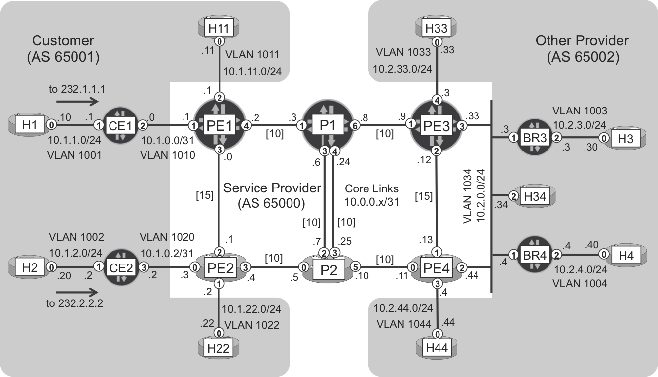
Figure 4-1. Internet Multicast topology
Note
All the hosts are simulated within a single IOS XR device or virtual machine (VM) called H. More specifically, each host is a VRF–lite inside H.
A simple ping is enough to generate multicast traffic. Let’s make host H1 send one packet per second toward 232.1.1.1, as shown in the following example:
Example 4-1. Generating IP Multicast traffic by using ping (IOS XR)
RP/0/0/CPU0:H#ping vrf H1 232.1.1.1 source 10.1.1.10
              count 100000 timeout 1
Type escape sequence to abort.
Sending 100000, 100-byte ICMP Echos to 232.1.1.1, timeout is 0s:
.............[...]
Tip
If you generate multicast packets from a Junos device, ensure that you use the bypass-routing, interface, and ttl ping options.
The previous ping fails. That’s expected given that there are no receivers yet: just let the ping run continuously in the background.
Next, let’s turn some hosts into dynamic multicast receivers. Here is a sample configuration for receiving host H11 at device H:
Example 4-2. Multicast receiver at H11 (IOS XR)
router igmp
 vrf H11
  interface GigabitEthernet0/0/0/0.1011
   join-group 232.1.1.1 10.1.1.10
!
This makes H11 begin to send dynamic IGMP Report messages, effectively subscribing to the (S, G) = (10.1.1.10, 232.1.1.1) flow. Let’s assume that H3, H4, H22, H33, H34, and H44 (in other words, every host except for H2) also subscribe to the same (S, G) flow.
Strictly speaking, the previous example is incomplete. For IOS XR to simulate a multicast end receiver, the interface must be turned on at the multicast-routing level first, and this has some implications.
Note
In Junos, this dynamic receiver emulation feature is only available in the ASM mode (protocols sap listen <group>). Additionally, both Junos and IOS XR support static subscriptions—ASM and SSM—at the receiver-facing interface of an LHR.
Signaling the Multicast Tree
After multicast sources and receivers are active, it’s time to signal the multicast tree. And for that, CEs and PEs need to run the multicast protocols shown here:
Example 4-3. Multicast routing configuration at PE1 (Junos)
protocols {
    igmp {
        interface ge-2/0/2.1011 version 3;
    pim {
        interface ge-2/0/2.1011;
        interface ge-2/0/1.1010;
}}
A similar configuration is applied to PE3, CE1, CE2, BR3, and BR4. For the moment, only the access (PE-H, PE-CE, and CE-H) interfaces are configured.
By default in Junos, an interface configured for PIM automatically runs IGMP on it, too. The default IGMP version is 2, and IGMP version 3 is required to process (S, G) Reports.
PIM is a router-to-router protocol, so strictly speaking the receiver-facing interface ge-2/0/2.1011 does not really need PIM. IGMP is enough on the last-hop interface. However, H11 might become a multicast sender at some point. Furthermore, as you will see soon in this chapter, enabling PIM on all of the router’s IP multicast access interfaces is considered a good practice for potential redundancy and loop detection.
The multicast traffic now flows end to end, thanks to the protocol exchange illustrated in Figure 4-2.
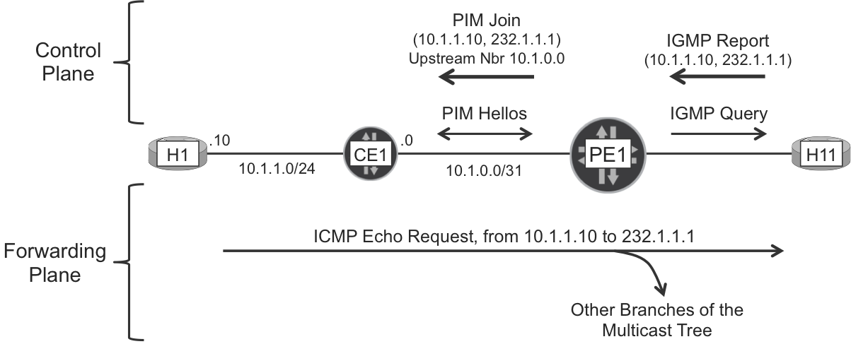
Figure 4-2. IGMP and PIM in action (SSM model)
Let’s look at the multicast routing configuration in IOS XR:
Example 4-4. Multicast routing configuration at PE2 (IOS XR)
multicast-routing
 address-family ipv4
  interface GigabitEthernet0/0/0/0.1020
   enable
  interface GigabitEthernet0/0/0/1.1022
   enable
The previous configuration actually enables PIM and IGMP on the specified PE-CE and PE-H interfaces.
IGMP signaling
The multicast tree is signaled in the upstream direction, from the receivers to the source. Let’s begin with the tree branch whose leaf is H11. The following capture, taken at PE1, shows the IGMP packet exchange between PE1 and H11.
Example 4-5. IGMP query (from PE1) and report (from H11)
juniper@PE1> monitor traffic interface ge-2/0/2.1011 no-resolve
             size 2000 extensive matching igmp
<timestamp> Out
  -----original packet-----
  00:50:56:8b:32:4a > 01:00:5e:00:00:01, ethertype 802.1Q (0x8100),
  length 54: vlan 1011, p 6, ethertype IPv4, (tos 0xc0, ttl 1,
  id 20138, offset 0, flags [none], proto: IGMP (2), length: 36,
  optlength: 4 ( RA )) 10.1.11.1 > 224.0.0.1: igmp query v3

<timestamp> In
  -----original packet-----
  IP (tos 0xc0, ttl 1, id 2772, offset 0, flags [none], proto: IGMP (2), length: 76,
  optlength: 4 ( RA )) 10.1.11.11 > 224.0.0.22: igmp v3 report [...]
  [gaddr 232.1.1.1 is_in { 10.1.1.10 }]
PE1 sends the IGMP Query to 224.0.0.1, the all-hosts link-local multicast address. H11 replies with an IGMP Report destined to 224.0.0.22, the all-IGMPv3-routers address. The information about the (S, G) subscriptions is in the payload of the IGMP Report.
Reverse Path Forwarding
PE1 further processes the IGMP Report by looking at the S address (10.1.1.10) and performing a unicast IP route lookup. This process of looking up the source is called Reverse Path Forwarding (RPF) and it’s a central concept in the multicast world.
Example 4-6. RPF at PE1 (Junos)
juniper@PE1> show route active-path 10.1.1.10

inet.0: 44 destinations, 53 routes (44 active, 0 holddown, 0 hidden)
+ = Active Route, - = Last Active, * = Both

10.1.1.0/24        *[BGP/170] 02:32:51, MED 100, localpref 100
                      AS path: 65001 I, validation-state: unverified
                    > to 10.1.0.0 via ge-2/0/1.1010

juniper@PE1> show multicast rpf 10.1.1.10
Multicast RPF table: inet.0 , 44 entries

10.1.1.0/24
    Protocol: BGP
    Interface: ge-2/0/1.1010
    Neighbor: 10.1.0.0
In a nutshell, multicast packets that arrive at the non-RPF interface are discarded.
By default, the unicast IP route lookup and the RPF lookup provide exactly the same result. The unicast and multicast topologies are then said to be congruent. If you want to make the unicast and multicast traffic follow different paths, it is also possible to make the topologies noncongruent. This is further discussed at the end of Chapter 5.
PIM signaling
CE1 and PE1 exchange PIM hello packets destined to 224.0.0.13, the all-PIM-routers link-local multicast address. Through that exchange, they become PIM neighbors.
Example 4-7. PIM neighbors at PE1 (Junos)
juniper@PE1> show pim neighbors
B = Bidirectional Capable, G = Generation Identifier
H = Hello Option Holdtime, L = Hello Option LAN Prune Delay,
P = Hello Option DR Priority, T = Tracking Bit

Instance: PIM.master
Interface        IP V Mode  Option     Uptime  Neighbor addr
ge-2/0/1.1010     4 2       HPLGT    02:40:25  10.1.0.0
From the perspective of PE1, the PIM neighbor CE1 is also the RPF upstream neighbor en route to the source. So, PE1 sends a PIM (S, G) Join message upstream to CE1:
Example 4-8. PIM (S, G) Join state from PE1 to CE1 (Junos)
juniper@PE1> show pim join inet detail
Instance: PIM.master Family: INET
R = Rendezvous Point Tree, S = Sparse, W = Wildcard

Group: 232.1.1.1
    Source: 10.1.1.10
    Flags: sparse,spt
    Upstream interface: ge-2/0/1.1010
    Downstream neighbors:
        Interface: ge-2/0/2.1011
The PIM (S, G) Join is actually a PIM Join/Prune packet. These messages contain a Join (add a branch) list, and a Prune (cut a branch) list. In this example, the receiver is turned on, so PE1 sends the Join/Prune packet with an empty Prune list. Such a PIM Join/Prune packet is commonly called a PIM Join. Example 4-9 shows the packet in detail.
Example 4-9. PIM (S, G) Join Packet from PE1 to CE1 (Junos)
juniper@PE1> monitor traffic interface ge-2/0/1.1010 no-resolve
             size 2000 detail matching pim
<timestamp> Out IP (tos 0xc0, ttl 1, id 36704, offset 0, no flags,
proto: PIM (103), length: 54) 10.1.0.1 > 224.0.0.13
  Join / Prune, cksum 0xd6dc (correct), upstream-neighbor: 10.1.0.0
    1 group(s), holdtime: 3m30s
      group #1: 232.1.1.1, joined sources: 1, pruned sources: 0
        joined source #1: 10.1.1.10(S)
Note
IGMP and PIM are hence soft-state protocols. In the IP Multicast world, all of the protocol messages (IGMP Query and Report, PIM Hello and Join/Prune, etc.) are refreshed periodically. By default, PIM Hello and Join/Prune are refreshed every 10 and 60 seconds, respectively.
As you can see, PIM messages are encapsulated as IP packets with protocol #103 and destination IP address 224.0.0.13. Because it is a link-local multicast IPv4 address, all of the PIM routers in the same VLAN would also process the packet. PE1 only has one neighbor in VLAN 1010, but what if there were more neighbors in the broadcast domain? How can PE1 indicate that the message is actually targeted to CE1? It does this via the upstream neighbor field in the PIM payload.
But, why is the PIM Join message sent to 224.0.0.13 if it’s targeted to CE1 only? PIM in a LAN is a complex topic and in some cases it is important that all the neighboring PIM routers LAN have full visibility of all the message exchanges. This prevents undesired traffic blackouts and duplication.
Multicast forwarding
Finally, CE1 is the FHR and after receiving the PIM Join/Prune packet, it just needs to forward the multicast traffic down to PE1, as shown in the following example:
Example 4-10. Multicast forwarding state at CE1 (Junos)
juniper@CE1> show multicast route inet detail
Instance: master Family: INET

Group: 232.1.1.1
    Source: 10.1.1.10/32
    Upstream interface: ge-0/0/1.1001
    Downstream interface list:
        ge-0/0/2.1010
    Session description: Source specific multicast
    Statistics: 0 kBps, 1 pps, 6064 packets
[...]
Note
This multicast route is not really a route. It is more accurately viewed as a forwarding cache entry.
Now that the source (H1) and the receiver (H11) are connected via the multicast tree, the multicast ping is successful: every echo request sent from H1 to 232.1.1.1 has one reply back, coming from H11 (10.1.11.11). If you don’t see the replies, you might be facing a corner-case condition in the dynamic receiver implementation: try to restart it by deleting and applying again the router igmp vrf H11 configuration at H (in two commits).
Classic Internet Multicast—Connecting Multicast Islands Across the Core
The tree now has one root (H1), one leaf (H11), and one single branch connecting them.
One-hop transit through the core (PE1-PE2)
Let’s add two more leaves to the tree:
-
H22 sends an IGMP (S, G) Report to PE2.
-
H2 sends an IGMP (S, G) Report to CE2, which sends a PIM (S, G) Join to PE2.
As a result, PE2 has the multicast (S, G) state depicted in the following example:
Example 4-11. Multicast RIB (IOS XR)
RP/0/0/CPU0:PE2#show mrib route 232.1.1.1
[...]
IP Multicast Routing Information Base
(10.1.1.10,232.1.1.1) RPF nbr: 0.0.0.0 Flags: RPF
  Up: 01:26:05
  Outgoing Interface List
    GigabitEthernet0/0/0/0.1020 Flags: F NS, Up: 01:26:00
    GigabitEthernet0/0/0/1.1022 Flags: F NS LI, Up: 01:26:05
The (S, G) entry is installed in PE2’s Multicast RIB (MRIB), but unfortunately the RPF neighbor is 0.0.0.0. In other words, RPF has failed. as shown in Example 4-12.
Example 4-12. Failed RPF at PE2 (IOS XR)
RP/0/0/CPU0:PE2#show pim rpf

Table: IPv4-Unicast-default
* 10.1.1.10/32 [200/100]
    via Null with rpf neighbor 0.0.0.0
Actually, PE2 has a valid BGP route toward 10.1.1.10, and its BGP next hop (172.16.0.11) is reachable via interface Gi 0/0/0/2. Why does RPF fail? Because PIM is not enabled in the core, so PE1 and PE2 are not PIM neighbors of each other.
In this classic MPLS-free example, the next step is enabling PIM on the core interfaces. When this is done, the new receivers are successfully connected to the source.
Example 4-13. Successful RPF at PE2 (IOS XR)
RP/0/0/CPU0:PE2#show pim neighbor GigabitEthernet 0/0/0/2
[...]
Neighbor Address  Interface              Uptime    Expires  DR pri

10.0.0.0          GigabitEthernet0/0/0/2 00:00:20  00:01:25 1
10.0.0.1*         GigabitEthernet0/0/0/2 00:00:20  00:01:26 1 (DR)

RP/0/0/CPU0:PE2#show pim rpf

Table: IPv4-Unicast-default
* 10.1.1.10/32 [200/100]
    via GigabitEthernet0/0/0/2 with rpf neighbor 10.0.0.0

RP/0/0/CPU0:PE2#show mrib route 232.1.1.1
[...]
(10.1.1.10,232.1.1.1) RPF nbr: 10.0.0.0 Flags: RPF
  Up: 01:50:26
  Incoming Interface List
    GigabitEthernet0/0/0/2 Flags: A, Up: 00:01:13
  Outgoing Interface List
    GigabitEthernet0/0/0/0.1020 Flags: F NS, Up: 01:50:21
    GigabitEthernet0/0/0/1.1022 Flags: F NS LI, Up: 01:50:26
At this point, the multicast tree has three leaves (H11, H22, and H2) connected to the root (H1), so the multicast ping receives three replies per request, as shown in Example 4-14.
Example 4-14. Successful multicast ping with three receivers
RP/0/0/CPU0:H#ping vrf H1 232.1.1.1 source 10.1.1.10 count 100000
Type escape sequence to abort.
Sending 100000, 100-byte ICMP Echos to 232.1.1.1, timeout is 2s:

Reply to request 0 from 10.1.11.11, 1 ms
Reply to request 0 from 10.1.2.20, 1 ms
Reply to request 0 from 10.1.22.22, 1 ms
Reply to request 1 from 10.1.11.11, 9 ms
Reply to request 1 from 10.1.2.20, 9 ms
Reply to request 1 from 10.1.22.22, 1 ms
[...]
One single copy of each packet traverses each link, including the PE1→PE2 connection. There are two replication stages: one at PE1, and another one at PE2.
With respect to the (10.1.1.10, 232.1.1.1) flow, PE1 and PE2 are popularly called sender PE and receiver PE, respectively. This is a per-flow role: one given PE can be a source PE for some flows, and a receiver PE for others. PE1 is not considered as a receiver PE even if it has a local receiver (H11), because the flow is not arriving from the core.
Note
In this chapter and in Chapter 5, the following terms are equivalent: root PE, ingress PE, and sender PE. Similarly, these terms are also synonyms: leaf PE, egress PE, and receiver PE.
Two-hop transit through the core (PE1-P1-PE3)
Let’s add one more leaf: H33. The LHR is now PE3, which as a PE has complete visibility of the customer BGP routes. Thanks to that, PE3 successfully performs an RPF lookup toward the source (10.1.1.10) and sends a PIM (S, G) Join to its upstream PIM neighbor: P1. So far, so good. However, P1 as a pure P-router does not have visibility of the BGP routes, so it fails to perform RPF toward the multicast source:
Example 4-15. Failed RPF at P1 (Junos)
juniper@P1> show route 10.1.1.10

inet.0: 33 destinations, 33 routes (33 active, 0 holddown, 0 hidden)
+ = Active Route, - = Last Active, * = Both

0.0.0.0/0          *[Static/5] 2w2d 05:08:19
                      Discard

juniper@P1> show pim join inet
Instance: PIM.master Family: INET
R = Rendezvous Point Tree, S = Sparse, W = Wildcard

Group: 232.1.1.1
    Source: 10.1.1.10
    Flags: sparse,spt
    Upstream interface: unknown (no neighbor)
But, how did the H2 and H22 receivers manage to join the multicast tree rooted at H1? Because the multicast branches that connects the root to H2 and H22 do not traverse any P-routers. Conversely, connecting H1 and H33 can be done only through a P-router; hence, the failure to signal the multicast branch end-to-end for H33.
How can you solve this problem? Actually, there are many ways—probably too many! Let’s see the different qualitative approaches to this challenge.
Signaling Join State Between Remote PEs
RPF failure in a transit router is a very similar problem to the classical one that motivated MPLS in Chapter 1. Now, it does not impact the forwarding of unicast data packets, but the propagation of PIM (S, G) Join states. The source S is an external unicast prefix that belongs to a different AS and is not reachable through the IGP. Chapter 1 proposed several ways to solve the unicast forwarding problem (without redistributing the external routes into the IGP), and all of them consisted of tunneling the user data packets. But here in the multicast case, it is the PIM (S, G) Join (a control packet), not the user data traffic, that needs to be tunneled. This opens the door to a more diverse set of design choices. Following are some possible strategies to signal Join state between remote PEs.
Note
This section focuses on the ways to solve RPF failures on transit routers. The discussion is independent of the service, which can be either Global Internet Multicast or Multicast VPN (MVPN). In practice, some of the approaches that follow are only implemented for MVPN.
Carrier IP Multicast Flavors
So let’s move from Classical IP Multicast to Carrier IP Multicast, which has tunneling capabilities in order to solve the multihop core challenge.
Table 4-1 lists six of the many dimensions that the multicast universe has.
| Service | Global Internet Multicast (S1), Multicast VPN (S2) |
| C-Multicast Architecture | None (A0), Direct Inter-PE (A1), Hop-by-Hop Inter-PE (A2), Out-of-Band (A3) |
| C-Multicast Inter-PE Signaling Protocol | None (C0), PIM (C1), LDP (C2), BGP (C3) |
| P-Tunnel Encapsulation | None (E0), GRE over IP Unicast (E1), GRE over IP Multicast (E2), MPLS (E3) |
| P-Tunnel Signaling Protocol | None (T0), PIM (T1), LDP (T2), RSVP-TE (T3), Routing Protocol with MPLS Extensions (T4) |
| P-Tunnel Layout | None (Y0), P2P (Y1), MP2P (Y2), P2MP (Y3), MP2MP (Y4) |
Note
The C- and P- prefixes stand for customer and provider, respectively. The classic IP Multicast model is purely C-Multicast. Conversely, Carrier IP Multicast models also have P- dimensions.
Every carrier multicast flavor has at least one element from each dimension. As you can imagine, not all the combinations make sense and each vendor supports only a subset of them. Although this book focuses on the combinations supported both by Junos and IOS XR, for completeness, noninteroperable combinations are also briefly discussed.
Tip
Print a copy of Table 4-1 and keep it as a reference as you read this book’s multicast chapters.
There are two types of service, depending on whether the multicast routing is performed on the global routing table or on a VRF. This chapter focuses on global services but it tactically borrows some examples that are only implemented for Multicast VPN.
This book considers three C-Multicast architectures:
-
In the Direct Inter-PE (A1) model, PE1 and PE3 establish a C-PIM adjacency through a bi-directional tunnel. This tunnel transports control and data C-Multicast packets.
-
In the Hop-by-Hop (A2) model, PE3 converts the upstream C-PIM Join state into a different message that P1 can process and send to PE1, which in turn converts it into C-PIM Join state. This architecture is also known as In-Band, or Proxy.
-
In the Out-of-Band (A3) model, PE3 signals the C-Join state to PE1 with a non-tunneled IP protocol. Like in the A1 model, P1 does not take any role in the C-Multicast control plane.
Don’t worry if these definitions do not make much sense yet. Keep them as a reference and they should be much clearer as you continue reading.
Note
In the terms of Table 4-1, the classic IP multicast model is: S1, A2, C1, E0, T0, Y0.
Direct Inter-PE Model—PE-to-PE PIM Adjacencies over Unicast IP Tunnels
In the terms of Table 4-1, this model is A1, C1, E1, T0, Y1. It is implemented by both Junos and IOS XR for S1 and S2.
This approach requires a unicast IP tunnel (e.g., GRE-based) between each pair of PEs. There is one PIM instance and it is running on the PEs only. This PIM context is often called C-PIM.
Let’s focus on the following tunnels: PE1→PE3 and PE3→PE1. PE1 and PE3 see this pair of GRE tunnels as a point-to-point interface that interconnects the two IP Multicast islands in a transparent manner. PE1 and PE3 exchange two types of multicast traffic over the GRE tunnels:
-
Control packets such as PIM Hello or (S, G) Join are destined to 224.0.0.13, a multicast (even if link-local, where the link is the GRE tunnel) address
-
Data packets of the active multicast user stream (10.1.1.10→232.1.1.1)
From the point of view of the GRE tunnels, there is no distinction between Control and Data. If PE1 needs to send a (Control or Data) multicast packet to PE3 over the PE1→PE3 GRE tunnel, it adds the following headers:
-
GRE header with Protocol Type = 0x0800 (IPv4).
-
IPv4 header with (Source, Destination) = (172.16.0.11, 172.16.0.33). In other words, the GRE tunnel’s endpoints are the primary loopback addresses of PE1 and PE3.
After receiving the tunneled packets, PE3 strips these two headers. The result is the original (Control or Data) multicast packet that PE1 had initially put into the tunnel. And the same logic applies to the packets that travel in the reverse direction: from PE3 to PE1.
How good is this model? Although you can use it in a tactical manner for limited or temporary deployments, you cannot consider it as a modern and scalable approach, for the same reasons why the Internet does not run over IP tunnels. The model is also affected by the following multicast-specific limitations:
-
If PE1 has two core uplink interfaces but it needs to send a multicast data packet to 1,000 remote PEs, PE1 must replicate the packet 999 times and send each one of the 1,000 copies into a different unicast GRE tunnel. This technique is called Ingress Replication, and it causes inefficient bandwidth consumption. When the multicast data packets are sent into the core, the main advantage of multicast (efficient replication tree) is simply lost.
-
The PEs establish PIM adjacencies through the GRE tunnels. The soft-state nature of PIM causes a periodic refresh of all the PIM packets (Hello, Join/Prune, etc.) at least once per minute. This background noise loads the control plane unnecessarily. Think for a moment on how the PEs exchange unicast routes: one BGP update through a reliable TCP connection, and that’s it (no periodic route refresh is required). In that sense, the multicast PE-to-PE protocol (PIM) is less scalable than the unicast protocol (BGP).
Whenever unicast GRE tunnels come into the multicast game, it is important to ensure that only the customer multicast traffic goes through them. The customer unicast traffic should travel in MPLS. This requirement for noncongruency is analyzed further at the end of Chapter 5.
Direct Inter-PE Model—PE-to-PE PIM Adjacencies over Multicast IP Tunnels
In the terms of Table 4-1, this model is A1, C1, E2, T1, [Y3, Y4]. It is implemented by both Junos and IOS XR for S2 only.
It is described in historic RFC 6037 - Cisco Systems’ Solution for Multicast in BGP/MPLS IP VPNs. Most people call it draft Rosen because draft-rosen-vpn-mcast was the precursor to RFC 6037.
In draft Rosen—implemented only for IP VPNs—each PE (e.g., PE1) is the root of at least one multicast GRE tunnel per VPN, called Multicast Distribution Tree (MDT). Why at least one and not just one? Let’s skip this question just for a moment, and think of each PE as the root of one MDT called the default MDT.
This model requires two different instances of PIM: C-PIM (where C stands for Customer) and P-PIM (where P stands for Provider). Note that C- and P- just represent different contexts. PIM is actually implemented in the same way—it is the same protocol after all:
-
C-PIM is the service instance of PIM and it runs at the edge: PE-to-CE, and PE-to-PE (the latter, through the GRE tunnels). It is used to signal the end-user multicast trees, in this example (10.1.1.10→232.1.1.1). So far, the PIM context used throughout this chapter has always been C-PIM. From the point of view of C-PIM, the core is just a LAN interface that interconnects all of the PEs. The PEs simply establish PIM adjacencies over the core, as they would do over any other interface.
-
P-PIM is the transport instance of PIM and runs on the core links only. It is used to build the Multicast GRE Provider Tunnels or P-Tunnels. The most popular P-PIM mode is SSM. One of the advantages of SSM here is that it makes Provider Group (P-G) assignment much simpler. Let’s suppose that PE1 and PE3 are the roots of P-Tunnels (172.16.0.11→P-G1) and (172.16.0.33→P-G3), respectively. P-G1 and P-G3 can be different, but they could also be the same. With SSM, as long as the sources are different, the multicast trees remain distinct even if G1 equals G3. This is especially important for data MDTs, discussed later in this section.
Note
P-PIM runs on the global routing instance (default VRF), whereas C-PIM runs on a (nondefault) VRF. So, the service is provided in the context of a VPN. And it can be the Internet Multicast service as long as it is provided within an Internet VPN.
Looking back at Table 4-1, P-PIM SSM corresponds to Y3 and P-PIM ASM to Y4.
Let’s suppose that each of the PEs in the core is the root of a P-Tunnel whose SSM P-Group is 232.0.0.100—the same one for simplicity, although it could be a different P-Group per root, too. PE1 receives the following P-PIM (S1, G) Joins from its P-PIM neighbors, where S1 = 172.16.0.11 and G = 232.0.0.1:
-
PE2 sends an (S1, G) Join directly to PE1.
-
PE3 sends an (S1, G) Join to P1 and then P1 sends an (S1, G) Join packets to PE1.
-
PE4 sends an (S1, G) Join to P2, then P2 sends an (S1, G) Join to P1, which is already sending (S1, G) Join packets to PE1.
In this way, PE1 is the root of a default MDT whose leaves are PE2, PE3, and PE4.
Likewise, PE1 is also a leaf of the remote PEs’ default MDTs. Indeed, PE1 sends the following P-PIM Joins: (172.16.0.22, 232.0.0.100) to PE2, (172.16.0.33, 232.0.0.100) to P1 en route to PE3, and (172.16.0.44, 232.0.0.100) to P1 en route to PE4.
This process ends up establishing an all-to-all LAN-like overlay that interconnects all the PEs with one another. PEs exchange two types of C-Multicast traffic over the default MDT:
-
Control packets like C-PIM Hello or C-PIM (S, G) Join are destined to 224.0.0.13, a multicast (even if link-local) address
-
Data packets of the active C-Multicast user stream (10.1.1.10→232.1.1.1)
From the point of view of the default MDT, there is no distinction between Control and Data. If PE1 needs to send a (Control or Data) C-Multicast packet to its neighbors over the default MDT, PE1 adds the following headers:
-
GRE header with Protocol Type = 0x0800 (IPv4)
-
IPv4 header with (Source, Destination) = (172.16.0.11, 232.0.0.100)
The tunneled packets arrive at all the other PEs, which strip the two headers. The result is the original (Control or Data) C-Multicast packet that PE1 had initially put into the default MDT.
PE1 is the root of its default MDT, and can optionally be the root of one or more data MDTs. What is a data MDT? Suppose that PE1 is the sender PE of a high-bandwidth C-Multicast (C-S, C-G) stream, and out of 1,000 remote PEs, only 10 of them have downstream receivers for (C-S, C-G). For bandwidth efficiency, it makes sense to signal a new MDT that is dedicated to transport that particular (C-S, C-G) only. This data MDT would only have 10 leaves: the 10 receiver PEs interested in receiving the flow.
Note
Default and Data MDTs are often called Inclusive and Selective Trees, respectively. Inclusive Trees include all the possible leaves, and Selective Trees select a specific leaf subset.
Note that the protocols described so far (C-PIM, P-PIM SSM, and GRE) are typically not enough to auto-discover the leaves of each MDT. Additional protocols are required and deployed to achieve this autodiscovery (AD) function. Which protocols? The answer varies depending on the implementation flavor. Using Cisco terminology (as of this writing):
- Rosen GRE
- Default MDT with P-PIM Any Source Multicast (ASM) does not require any extra protocols, because the P-Source AD function is performed by P-PIM (source discovery in PIM ASM is discussed in Chapter 15). As for Data MDTs, they are signaled with User Datagram Protocol (UDP) packets that are exchanged in the Default MDT.
- Rosen GRE with BGP AD
- Default MDT with P-PIM SSM requires a new multiprotocol BGP address family for (P-S, P-G) AD. As for Data MDTs, they can be signaled either by using BGP or UDP.
Note
Cisco documentation associates each carrier multicast flavor with a profile number. For example, Rosen GRE is MVPN Profile 0, and Rosen GRE with BGP AD is MVPN Profile 3.
Further details of Rosen GRE implementation and interoperability are beyond the scope of this book, as we’re focusing on MPLS and not GRE. Let’s be fair: draft Rosen has been the de facto L3 Multicast VPN technology for two decades, and it has solved the business requirements of many customers. But, as time moves on, it is being replaced by next-generation models.
Wrapping up, let’s take a look at the pros and cons of this model:
-
Pro: an MDT is actually a (provider) multicast tree that facilitates the efficient replication of multicast data. If PE1 has two core uplink interfaces and it needs to send a multicast data packet to 1,000 remote PEs, PE1 replicates the packet at most once and sends at most one copy of the packet out of each core uplink. Also, this model implements data MDT for an even more efficient distribution.
-
Con: C-PIM in a LAN is complex and noisy. If PE3 sends a C-PIM Join to PE1, all of the other PEs in the VPN receive it and look into it. As you have seen previously, PIM Join/Prune messages are sent to 224.0.0.13 and are periodically refreshed. This makes the solution less scalable and robust in the control plane.
-
Finally, this model does not provide total forwarding-plane flexibility. There are two P-Tunnel types available: PIM/GRE and MP2MP mLDP (coming next). None of them can benefit from MPLS features such as Traffic Engineering.
Warning
Before moving on, let’s first remove PIM from all of the core links because P-PIM is not needed anymore. From now on, the core is MPLS territory!
Direct Inter-PE Model—PE-PE PIM Adjacencies over MPLS Label-Switched Paths
In the terms of Table 4-1, this model is A1, C2, E3, T2, Y4. It is implemented only by IOS XR and for S2 only.
PIM is designed for bidirectional links. When R1 sends a PIM Join to R2 over link L, the multicast traffic must flow from R2 to R1 over the same link L. However, MPLS Label-Switched Paths (LSPs) are unidirectional—or are they? Actually, there is one type of LSP that is bi-directional. It is called Multipoint-to-Multipoint LSP (MP2MP LSP) and it’s one of the two LSP types described in RFC 6388 - Label Distribution Protocol Extensions for Point-to-Multipoint and Multipoint-to-Multipoint Label Switched Paths. With any of these (P2MP or MP2MP) extensions, LDP is often referred to as Multipoint LDP (mLDP). Paraphrasing the RFC:
An MP2MP LSP [...] consists of a single root node, zero or more transit nodes, and one or more Leaf LSRs acting equally as an ingress or egress LSR.
In a nutshell, MP2MP LSPs have a central (so-called root) LSR, where all the branches meet. The PEs sit at the leaves and exchange with their LDP neighbors two types of multipoint (MP) FEC Label Mappings: up, for user traffic flowing from a leaf to the root, and down, for user traffic flowing from the root to a leaf. From a service perspective, the MP2MP LSP emulates a bidirectional LAN interconnecting the PEs, and with no learning mechanism to reduce flooding. Any packet put in an MP2MP LSP reaches all of the leaves. In that sense, the MP2MP LSP is a Default MDT or Inclusive Tree.
As of this writing, Cisco calls this model Rosen mLDP, as it has many similarities to Rosen GRE. Cisco documentation uses the name Rosen to tag a wide variety of MVPN profiles. Some of them are similar to draft Rosen (draft-rosen-vpn-mcast), whereas others are not. So, this tag does not really provide a hint with respect to the underlying technology.
In both Rosen GRE and Rosen mLDP, the PEs build C-PIM adjacencies over the Default MDT. Therefore, they both rely on the implementation of C-PIM on a LAN. Last but not least, they both require additional mechanisms to auto-discover the leaves of Default and/or Data MDTs.
Note
Data MDTs are P2MP, unlike the Default MDT, which is MP2MP.
The main difference between Rosen GRE and Rosen mLDP lies in the way the C-PIM messages and C-Multicast packets are exchanged over the Default MDT: through IP or MPLS tunnels, respectively. In Rosen mLDP, C-PIM Joins are encapsulated in MPLS, and they flow in the opposite direction to C-Multicast traffic. You can compare Rosen GRE to Rosen mLDP by replacing P-PIM with LDP, and GRE with MPLS.
Neither Rosen GRE nor Rosen mLDP are further covered in this book. The first is not based on MPLS, and the second is not interoperable as of today. Both models rely on establishing PE-PE C-PIM adjacencies across the core.
Beyond the Direct Inter-PE Model—Not Establishing PE-PE PIM Adjacencies
Previous models’ assessment shows that tunneling C-PIM between PEs is not particularly scalable. In the early 2000s, Juniper and Cisco began to define new frameworks to signal and transport multicast traffic across an MPLS backbone. At the time, this new set of paradigms was called Next-Generation or NG, but right now it is simply state-of-the-art technology. Although many people continue to call it NG, this book does not.
These modern frameworks leave PIM running on PE-CE and PE-Host links only. However, the PEs no longer establish C-PIM adjacencies with one another. Instead, a scalable carrier-class protocol signals inter-PE C-Multicast information. There are basically two such protocols: BGP and LDP. Both of them are capable of encoding C-Multicast state.
Out-of-Band Model
When BGP is used to signal C-Multicast Join state, the service and the transport planes are loosely coupled. Thanks to certain techniques that are described in Chapter 5, BGP virtually supports all of the dynamic P-Tunnel technologies listed in Table 4-1.
Let’s consider the particular case in which LDP is the P-Tunnel signaling protocol. In the terms of Table 4-1, this model is A3, C3, E3, T2, [Y2, Y3, Y4]. The role of LDP in this case is to build the LSPs that transport the multicast data. BGP fully takes care of the PE-to-PE service C-Multicast signaling. In that sense, the service plane (BGP) is not tightly coupled to the transport plane (LDP here). BGP performs Out-of-Band C-Multicast signaling. This model provides great flexibility in the P-Tunnel choice, and it relies on a rich signaling mechanism, which is covered later in Chapter 5.
Hop-by-Hop Inter-PE model
When LDP is used (instead of BGP) to signal C-Multicast Join state, the service and the transport planes are tightly coupled: LDP signals both at the same time, thanks to special FEC types. This is In-Band C-Multicast signaling, which means that the service and the transport planes are blended.
This model is less flexible and scalable than the out-of-band architecture, but also simpler to understand, so let’s use it for the first Multicast over MPLS illustrated example in this book. Finally!
Internet Multicast over MPLS with In-Band Multipoint LDP Signaling
This section illustrates the P2MP part of RFC 6826 - Multipoint LDP In-Band Signaling for Point-to-Multipoint and Multipoint-to-Multipoint Label Switched Paths.
In the terms of Table 4-1, this model is S1, A2, C2, E3, T2, Y3. In Cisco documentation, it is called Global Inband. It is the simplest way to deploy dynamic Multicast over MPLS. Although it brings easy operation and deployment, this carrier multicast flavor also has some limitations:
-
It creates C-Multicast label state at the core LSRs, breaking one of the main benefits of MPLS: reducing the state by not propagating customer routes to the P-routers.
-
It does not have P-Tunnel flexibility (it is restricted to LDP only).
-
It does not yet support Inclusive Tunnels (default MDTs).
Multipoint LDP
Multipoint LDP (mLDP) is not a new protocol; rather, it is a set of LDP extensions and procedures. PE1 and PE2 establish one single LDP session, and they use it to exchange label mappings for all the FEC elements. These include good old IPv4 prefixes (as in plain LDP) and, in addition, the Multipoint FEC elements; all advertised in the same LDP session.
Tip
Use the policy framework in Junos and IOS XR to select which FECs you want to advertise over the LDP session. For example, you might want to use LDP only for P2MP FECs, not for IPv4 Unicast FECs.
LDP is called mLDP if the neighbors negotiate special MP capabilities. More specifically, a neighbor supporting the P2MP capability (0x0508) can signal P2MP FEC elements over a (m)LDP session.
Let’s begin with a scenario in which LDP is configured on all the interfaces (see Chapter 2). Example 4-16 shows the incremental mLDP configuration in Junos.
Example 4-16. mLDP configuration (Junos)
protocols {
    ldp p2mp;
}
Example 4-17 presents the configuration in IOS XR.
Example 4-17. mLDP configuration (IOS XR)
mpls ldp
 mldp
Note
It is a good practice in both Junos and IOS XR to configure mLDP make-before-break in order to minimize traffic loss upon link recovery. The details are outside the scope of this book.
As a result of this configuration, LDP peers negotiate the P2MP capability. Let’s see the negotiation between PE1 (Junos) and PE2 (IOS XR): they both have in common the P2MP capability:
Example 4-18. LDP capability negotiation (Junos and IOS XR)
juniper@PE1> show ldp session 172.16.0.22 detail
[...]
  Capabilities advertised: p2mp, make-before-break
  Capabilities received: p2mp

RP/0/0/CPU0:PE2#show mpls ldp neighbor 172.16.0.11:0 detail
[...]
  Capabilities:
    Sent:
      0x508  (MP: Point-to-Multipoint (P2MP))
      0x509  (MP: Multipoint-to-Multipoint (MP2MP))
      0x50b  (Typed Wildcard FEC)
    Received:
      0x508  (MP: Point-to-Multipoint (P2MP))
For now, the LDP session only signals the classic IPv4 prefix FEC elements. For the moment, no P2MP FEC elements are being advertised on the LDP sessions because there is no service requiring a multipoint LSP yet. This is about to change.
Note
You need to configure mLDP on all the LSRs and LERs.
In-Band Signaling
At this point, PE2, PE3, and PE4 have upstream PIM Join state pointing to PE1, but RPF is failing because PIM has been removed from the core links. In C- and P- terminology, P-PIM is no longer running and C-PIM needs to rely on mLDP in order to extend the multicast tree through the core. However, C-PIM does not know that it can rely on mLDP. Yet.
Later in this chapter, you will see the configuration (see Example 4-19 and Example 4-26) that allows the automatic conversion of C-PIM Join state into LDP P2MP FECs. This triggers the creation of a P2MP LSP rooted at PE1 and with three leaves (PE2, PE3, and PE4). The P2MP LSP is built by mLDP, and the signaling actually goes in the upstream direction: from the leaves toward the root (PE1). In contrast, the C-Multicast data is tunneled downstream, from the root to the leaves.
You can use Figure 4-3 as a guide for the following mLDP walkthrough.
Note
For the remainder of this chapter, the links PE1-PE2 and PE3-PE4 have their IS-IS metrics raised to 100. So, in the absence of link failures, all the inter-PE shortest paths go through P-routers.
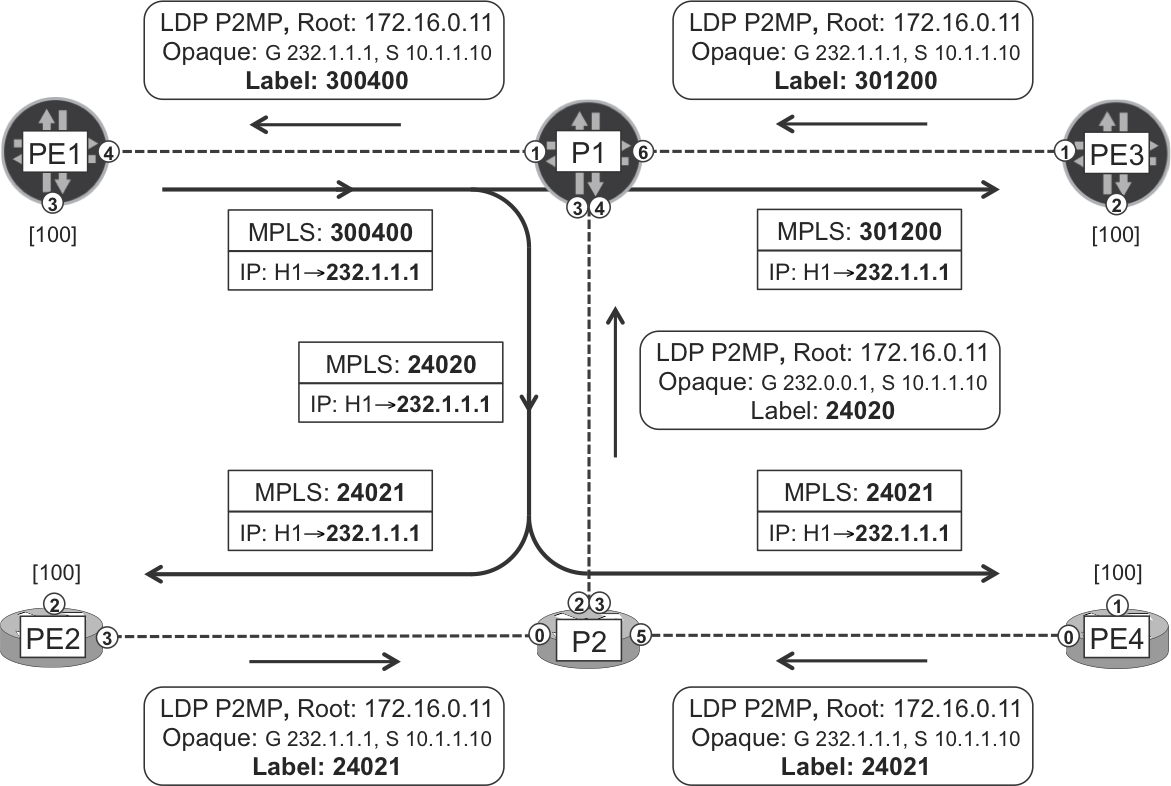
Figure 4-3. mLDP P2MP LSPs—In-Band signaling and forwarding
Assume that all the hosts back in Figure 4-1, with the exception of source H1, are subscribed to the (10.1.1.10, 232.1.1.1) multicast flow. In other words: H2, H3, H4, H22, H33, H34, and H44 are all C-Multicast receivers.
Signaling Join state from an egress PE that runs Junos
The folowing Junos configuration links C-PIM to mLDP at the Junos PEs:
Example 4-19. mLDP In-Band configuration at the PEs (Junos)
protocols {
    pim mldp-inband-signalling;
}
Note
This configuration is only needed on the (ingress and egress) PEs. Pure P-routers such as P1 and P2 do not need it, because they do not even run PIM.
After clearing the C-PIM Join state at PE3—by using the command clear pim join—the multicast ping from H1 to 232.1.1.1 begins to receive replies from H3, H4, and H33.
Warning
Use the clear pim join command with caution. This command is typically disruptive for the established multicast flows. Try to be specific with respect to the particular (S, G) that you want to clear.
Letl’s see how this PE1→PE3 branch of the multicast tree is signaled through the core. The egress PE (PE3) knows that the C-Multicast source 10.1.1.10 is beyond PE1.
Example 4-20. RPF resolution at egress PE—PE3 (Junos)
juniper@PE3> show route 10.1.1.10 detail active-path
[...]
         Protocol next hop: 172.16.0.11

juniper@PE3> show pim source inet
Instance: PIM.master Family: INET

Source 10.1.1.10
    Prefix 10.1.1.0/24
    Upstream protocol MLDP
    Upstream interface Pseudo MLDP
    Upstream neighbor MLDP LSP root <172.16.0.11>
Thanks to the configuration just applied, PE3’s upstream C-PIM Join state can be resolved via Multicast Label Distribution Protocol (mLDP), as shown in Example 4-21.
Example 4-21. Upstream C-PIM Join state at egress PE—PE3 (Junos)
juniper@PE3> show pim join inet detail
Instance: PIM.master Family: INET
R = Rendezvous Point Tree, S = Sparse, W = Wildcard

Group: 232.1.1.1
    Source: 10.1.1.10
    Flags: sparse,spt
    Upstream protocol: MLDP
    Upstream interface: Pseudo MLDP
    Downstream neighbors:
        Interface: ge-2/0/3.1034
        Interface: ge-2/0/4.1033
From the forwarding plane perspective, the (downstream) path is PE1→PE3, but it must be signaled the other way around: from PE3 to PE1. In other words, signaling takes place upstream from the leaf to the root. PE3 is not directly connected to PE1, so PE3 (the egress PE) needs to find the RPF neighbor toward PE1 (the root).
Example 4-22. RPF lookup at egress PE—PE3 (Junos)
juniper@PE3> show route 172.16.0.11 table inet.0

inet.0: 43 destinations, 51 routes (43 active, 0 holddown, 0 hidden)
+ = Active Route, - = Last Active, * = Both

172.16.0.11/32     *[IS-IS/18] 04:37:38, metric 20
                    > to 10.0.0.8 via ge-2/0/1.0
Now, PE3 builds a P2MP FEC element, maps a label to it, and advertises the Label Mapping only to P1. Why P1? Because it is the RPF neighbor—and LDP neighbor—toward the root (PE1). This targeted advertisement is totally different from the promiscuous Label Mapping distribution of IPv4 Prefix FEC elements, depicted in Figure 2-3 and Figure 2-4. In the P2MP case, the downstream LSR performs a route lookup before advertising the Label Mapping, and as a result, only the RPF neighbor receives it.
Example 4-23. P2MP FEC signaling from egress PE—PE3 (Junos)
juniper@PE3> show ldp p2mp fec
LDP P2MP FECs:
 P2MP root-addr 172.16.0.11, grp: 232.1.1.1, src: 10.1.1.10
  Fec type: Egress (Active)
  Label: 301200

juniper@PE3> show ldp database p2mp
Input label database, 172.16.0.33:0--172.16.0.1:0
Labels received: 8

Output label database, 172.16.0.33:0--172.16.0.1:0
Labels advertised: 19
  Label   Prefix
 301200   P2MP root-addr 172.16.0.11, grp: 232.1.1.1, src: 10.1.1.10

Input label database, 172.16.0.33:0--172.16.0.44:0
Labels received: 19

Output label database, 172.16.0.33:0--172.16.0.44:0
Labels advertised: 18
Let’s interpret the new FEC element. The format of MP (P2MP and MP2MP) FEC elements is described in RFC 6388 - LDP Extensions for Point-to-Multipoint and Multipoint-to-Multipoint Label Switched Paths, which we paraphrase here:
The P2MP FEC Element consists of the address of the root of the P2MP LSP and an opaque value. [...] The opaque value is unique within the context of the root node. The combination of (Root Node Address type, Root Node Address, Opaque Value) uniquely identifies a P2MP LSP within the MPLS network.
Back to the example, the P2MP Root Address is 172.16.0.11 (PE1’s loopback address) and the Opaque Value is: group 232.1.1.1, source 10.1.1.10. As you can see, the FEC element used to build this P2MP LSP also contains C-Multicast information, namely the C-Group and the C-Source. This is precisely what In-Band means. But this information is encoded in an opaque value, which means that the transit LSRs do not need to understand it: only the root does.
When P1 receives this P2MP FEC element, it only looks at its root address (172.16.0.11) and, of course, at the label. P1 performs an RPF check, allocates a new label, and sends a P2MP Label Mapping to its RPF neighbor toward the root, PE1.
Example 4-24. mLDP P2MP FEC signaling from transit P—P1 (Junos)
juniper@P1> show ldp p2mp fec
LDP P2MP FECs:
 P2MP root-addr 172.16.0.11, grp: 232.1.1.1, src: 10.1.1.10
  Fec type: Transit (Active)
  Label: 300400

juniper@P1> show ldp database session 172.16.0.11 p2mp
Input label database, 172.16.0.1:0--172.16.0.11:0
Labels received: 9

Output label database, 172.16.0.1:0--172.16.0.11:0
Labels advertised: 7
  Label  Prefix
 300400   P2MP root-addr 172.16.0.11, grp: 232.1.1.1, src: 10.1.1.10
Unlike P1, the ingress PE (PE1) is the root, so it looks into the MP opaque value, which contains C-Multicast state. Indeed, PE1 converts the downstream mLDP FEC into upstream C-PIM Join state. The latter already exists due to the local receiver H11, so the mLDP FEC simply triggers an update of the outgoing interface list.
Example 4-25. Upstream C-PIM Join state at ingress PE—PE1 (Junos)
juniper@PE1> show pim join inet detail
Instance: PIM.master Family: INET
R = Rendezvous Point Tree, S = Sparse, W = Wildcard

Group: 232.1.1.1
    Source: 10.1.1.10
    Flags: sparse,spt
    Upstream interface: ge-2/0/1.1010
    Downstream neighbors:
        Interface: ge-2/0/2.1011
        Interface: Pseudo-MLDP
Signaling Join state from an egress PE that runs IOS XR
The IOS XR configuration that links C-PIM to mLDP at PE2 is shown in Example 4-26.
Example 4-26. mLDP In-Band Configuration at PE2 (IOS XR)
prefix-set PR-REMOTE-SOURCES
  10.1.1.0/24 eq 32,
  10.2.0.0/16 eq 32
end-set
!
route-policy PL-MLDP-INBAND
  if source in PR-REMOTE-SOURCES then
    set core-tree mldp-inband
  else
    pass
  endif
end-policy
!
router pim
 address-family ipv4
  rpf topology route-policy PL-MLDP-INBAND
!
multicast-routing
 address-family ipv4
  mdt mldp in-band-signaling ipv4
!
PE4 is configured in a similar way, with just some adjustments in the prefix-set. Like in Junos, this configuration is only required at the PEs, not at the Ps. After clearing the C-PIM Join state at PE2 and PE4—by using the command clear pim ipv4 topology—the multicast ping from H1 to 232.1.1.1 begins to receive replies from H2, H22, and H44.
Warning
Use the clear pim ipv4 topology command with caution. This command is typically disruptive for the established multicast flows. Try to be specific with respect to the particular (S, G) that you want to clear.
Let’s see how these branches of the multicast tree are signaled through the core. Actually, one of the egress PEs (PE2) acts as a branching point, so the H1→H2 and H1→H22 paths actually share the same subpath (PE1→PE2) in the core.
Following is the C-PIM upstream Join state at PE2. Remember that the PE1-PE2 link has a high IS-IS metric value, so the shortest PE2→PE1 path goes via P2 and P1.
Example 4-27. Upstream C-PIM Join at egress PE—PE2 (IOS XR)
RP/0/0/CPU0:PE2#show mrib route 232.1.1.1

IP Multicast Routing Information Base
[...]
(10.1.1.10,232.1.1.1) RPF nbr: 10.0.0.5 Flags: RPF
  Up: 01:00:38
  Incoming Interface List
    Imdtdefault Flags: A LMI, Up: 01:00:38
  Outgoing Interface List
    GigabitEthernet0/0/0/0.1020 Flags: F NS, Up: 01:00:38
    GigabitEthernet0/0/0/1.1022 Flags: F NS LI, Up: 01:00:38
The imdtdefault interface is the internal “glue” between the C-PIM and the mLDP domains at PE2. Don’t be confused by the name: this mLDP LSP is a data MDT (selective tree). Now, the C-PIM upstream Join state triggers the creation and signaling of a P2MP FEC label mapping that PE2 sends up to P2.
Example 4-28. P2MP FEC signaling from egress PE—PE2 (IOS XR)
RP/0/0/CPU0:PE2#show mpls mldp database
mLDP database
LSM-ID: 0x00001   Type: P2MP   Uptime: 01:08:29
  FEC Root           : 172.16.0.11
  Opaque decoded     : [ipv4 10.1.1.10 232.1.1.1]
  Upstream neighbor(s) :
    172.16.0.2:0 [Active] Uptime: 00:12:26
      Local Label (D) : 24021
  Downstream  client(s):
    PIM MDT            Uptime: 01:08:29
      Egress intf     : Imdtdefault
      Table ID        : IPv4: 0xe0000000
      RPF ID          : 3
P2 receives P2MP FEC label mappings from PE2 and PE4, which are then aggregated into one single label mapping that P2 signals upstream to P1.
Example 4-29. P2MP FEC signaling at Transit P—P2 (IOS XR)
RP/0/0/CPU0:P2#show mpls mldp database
mLDP database
LSM-ID: 0x00003   Type: P2MP   Uptime: 00:39:07
  FEC Root           : 172.16.0.11
  Opaque decoded     : [ipv4 10.1.1.10 232.1.1.1]
  Upstream neighbor(s) :
    172.16.0.1:0 [Active] Uptime: 00:39:07
      Local Label (D) : 24020
  Downstream  client(s):
    LDP 172.16.0.22:0  Uptime: 00:39:07
      Next Hop         : 10.0.0.4
      Interface        : GigabitEthernet0/0/0/0
      Remote label (D) : 24021
    LDP 172.16.0.44:0  Uptime: 00:37:55
      Next Hop         : 10.0.0.11
      Interface        : GigabitEthernet0/0/0/5
      Remote label (D) : 24021
Note
In Example 4-29, the remote label value 24021 happens to be the same in both of the downstream branches. This is just a typical MPLS coincidence; the labels also could have had different values.
This is the control-plane view of a branching point: two downstream branches (P2→PE2 and P2→PE4) are merged into a single upstream branch (P1→P2). In the forwarding plane, the process is the opposite: a packet arriving on P2 from P1 is replicated toward PE2 and PE4. Let’s examine the life of a C-Multicast packet.
Life of a C-Multicast Packet in an mLDP P2MP LSP
After analyzing the control plane, let’s focus on the forwarding plane.
Ingress PE
PE1 replicates each incoming (10.1.1.10, 232.1.1.1) C-Multicast packet and sends one copy down to the directly connected receiver H11, and one more copy—encapsulated in MPLS—down the PE1-P1 core link, as shown in Example 4-30.
Example 4-30. mLDP P2MP LSP forwarding at the ingress PE—PE1 (Junos)
1     juniper@PE1> show multicast route detail
2     Instance: master Family: INET
3
4     Group: 232.1.1.1
5         Source: 10.1.1.10/32
6         Upstream interface: ge-2/0/1.1010
7         Downstream interface list:
8             ge-2/0/4.0 ge-2/0/2.1011
9         Session description: Source specific multicast
10        Statistics: 0 kBps, 1 pps, 8567 packets
11        Next-hop ID: 1048581
12        Upstream protocol: PIM
13
14    juniper@PE1> show route table inet.1 match-prefix "232.1.1.1*"
15
16    inet.1: 4 destinations, 4 routes (4 active, 0 holddown, 0 hidden)
17    + = Active Route, - = Last Active, * = Both
18
19    232.1.1.1,10.1.1.10/64*[PIM/105] 07:08:35
20                          to 10.0.0.3 via ge-2/0/4.0, Push 300400
21                          via ge-2/0/2.1011
22
23    juniper@PE1> show route forwarding-table destination 232.1.1.1
24                 table default extensive
25    Destination:  232.1.1.1.10.1.1.10/64
26      Route type: user
27      Route reference: 0                   Route interface-index: 332
28      Multicast RPF nh index: 0
29      Flags: cached, check incoming interface, [...]
30      Next-hop type: indirect        Index: 1048581  Reference: 2
31      Nexthop:
32      Next-hop type: composite       Index: 595      Reference: 1
33      # Now comes the list of core (MPLS) next hops
34      Next-hop type: indirect        Index: 1048577  Reference: 2
35      Nexthop:
36      Next-hop type: composite       Index: 592      Reference: 1
37      Nexthop: 10.0.0.3
38      Next-hop type: Push 300400     Index: 637      Reference: 2
39      Load Balance Label: None
40      Next-hop interface: ge-2/0/4.0
41      # Now comes the list of access (IPv4) next hops
42      Next-hop type: indirect        Index: 1048591  Reference: 2
43      Nexthop:
44      Next-hop type: composite       Index: 633      Reference: 1
45      Next-hop type: unicast         Index: 1048574  Reference: 3
46      Next-hop interface: ge-2/0/2.1011
All of the previous commands simply show different stages of a multicast forwarding cache entry. The inet.1 auxiliary Routing Information Base (RIB) is actually a multicast cache whose entries populate the forwarding table (the Forwarding Information Base [FIB]). There is a deep level of indirection in the Junos next-hop structures. In practice, you can think of the composite next hop as an action. In the case of multicast routes, this action is replicate. You can find a full discussion about composite next hops applied to unicast in Chapter 20.
Look at line 37 in Example 4-30. One copy of the C-Multicast packet is encapsulated in MPLS and then into Ethernet. The destination MAC address of the Ethernet frame is the unicast MAC address associated to 10.0.0.3 (P1), typically resolved via ARP.
Note
Multicast over MPLS over Ethernet is transported in unicast frames.
This is an important advantage for scenarios in which the core link, despite being logically point-to-point, transits an underlying multipoint infrastructure. For example, AS 65000 may buy multipoint L2VPN services to an external SP and use this L2 overlay to implement its own core links. From the perspective of AS 65000, these are point-to-point core links, but behind the scenes multicast Ethernet frames are flooded through the multipoint L2VPN at the transport provider network. This reasoning highlights the advantage of encapsulating the C-Multicast packets in unicast MPLS-over-Ethernet frames. L2VPN services are further discussed in Chapters Chapter 6, Chapter 7 and Chapter 8.
Finally, you can ignore the term unicast in Example 4-30, line 45. Its meaning is fully explained in Chapter 20 and it has nothing to do with the classical notion of unicast.
Due to the currently configured IGP metric scheme—inter-PE links have a higher metric (100)—PE1 only sends one copy of the C-Multicast packet into the core. If the IGP metrics were set back to the default values, PE1 would send one copy to P1 and another copy to PE2. In other words, nothing prevents an ingress PE from being a replication point of a P2MP LSP if the topology requires it.
Note
In this example, the ingress PE (PE1) runs Junos. If the multicast ping is sourced from H2, the ingress PE (PE2) runs IOS XR, and the results are successful and symmetrical to those shown here.
Transit P-router running Junos
When it arrives to P1, the MPLS packet is further replicated in two copies: one goes to PE3, and another one to P2, as shown in Example 4-31.
Example 4-31. mLDP P2MP LSP forwarding at a transit PE—P1 (Junos)
juniper@P1> show ldp p2mp path
P2MP path type: Transit/Egress
  Output Session (label): 172.16.0.11:0 (300400) (Primary)
  Input Session (label): 172.16.0.33:0 (301200)
                         172.16.0.2:0 (24020)
  Attached FECs:  P2MP root-addr 172.16.0.11,
                  grp: 232.1.1.1, src: 10.1.1.10 (Active)

juniper@P1> show route forwarding-table label 300400 extensive
Routing table: default.mpls [Index 0]
MPLS:

Destination:  300400
  Route type: user
  Route reference: 0              Route interface-index: 0
  Multicast RPF nh index: 0
  Flags: sent to PFE
  Next-hop type: indirect         Index: 1048582  Reference: 2
  Nexthop:
  Next-hop type: composite        Index: 602      Reference: 1
  # Now comes the replication towards PE3
  Nexthop: 10.0.0.9
  Next-hop type: Swap 301200      Index: 594      Reference: 2
  Load Balance Label: None
  Next-hop interface: ge-2/0/6.0
  # Now comes the replication towards P2
  Next-hop type: unilist          Index: 1048581  Reference: 2
  # Now comes the first P1-P2 link for load balancing
  Nexthop: 10.0.0.7
  Next-hop type: Swap 24020       Index: 596      Reference: 1
  Load Balance Label: None
  Next-hop interface: ge-2/0/3.0  Weight: 0x1
  # Now comes the second P1-P2 link for load balancing
  Nexthop: 10.0.0.25
  Next-hop type: Swap 24020       Index: 597      Reference: 1
  Load Balance Label: None
  Next-hop interface: ge-2/0/4.0  Weight: 0x1
If you look carefully at Example 4-31, there is a new type of next hop called unilist. It means that the single copy of the packet that is sent down to P2 needs to be load balanced—not replicated—across the two P1-P2 links. This single copy is sent down the first or down the second link, depending on the results of the packet hash computation (see “LDP and Equal-Cost Multipath” if this language does not sound familiar to you). The fact that the Weight is 0x1 in both links means that they are both available for load balancing. Hence, in Junos, mLDP natively supports Equal-Cost Multipath (ECMP) across parallel links.
Transit P-router running IOS XR
P2 further replicates the packet down to PE2 and PE4, as illustrated in the folowing example:
Example 4-32. mLDP P2MP LSP forwarding at a transit PE—P2 (IOS XR)
RP/0/0/CPU0:P2#show mpls forwarding labels 24020
Local  Outgoing  Prefix         Outgoing   Next Hop    Bytes
Label  Label   or ID          Interface             Switched
------ ------- -------------- ---------- ---------- --------
24020  24021   MLDP: 0x00003  Gi0/0/0/0  10.0.0.4   2170
       24021   MLDP: 0x00003  Gi0/0/0/5  10.0.0.11  2170
Egress PE running Junos
PE3 pops the MPLS label and replicates the resulting IPv4 multicast packets toward the two receiver ACs, as you can see in Example 4-33.
Note
There is no Penultimate Hop Popping (PHP) for P2MP LSPs. In this chapter’s Global Internet Multicast case, this is important because the core links should not transport native user multicast packets. As for the Multicast VPN case, it is also important but for a different reason, which is discussed in Chapter 5.
Example 4-33. mLDP P2MP LSP forwarding at an egress PE—PE3 (Junos)
juniper@PE3> show route forwarding-table label 301200 extensive
Routing table: default.mpls [Index 0]
MPLS:

Destination:  301200
  Route type: user
  Route reference: 0                   Route interface-index: 0
  Multicast RPF nh index: 0
  Flags: sent to PFE
  Next-hop type: indirect              Index: 1048577  Reference: 2
  Nexthop:
  Next-hop type: composite             Index: 601      Reference: 1
  # Now comes the replication towards VLAN 1034 [...]
  Next-hop type: Pop                   Index: 597      Reference: 2
  Load Balance Label: None
  Next-hop interface: ge-2/0/3.1034
  # Now comes the replication towards H33 [...]
  Next-hop type: Pop                   Index: 600      Reference: 2
  Load Balance Label: None
  Next-hop interface: ge-2/0/4.1033
Unicast next hops have been stripped from Example 4-33 because they are misleading: multicast MAC addresses are calculated with a mathematical rule; they are not resolved via ARP.
Egress PE running IOS XR
Let’s see how PE4 pops the MPLS label and sends the IPv4 multicast packet to H44 only.
Example 4-34. mLDP P2MP LSP Forwarding at an egress PE–PE4 (IOS XR)
RP/0/0/CPU0:PE4#show mrib route 10.1.1.10 232.1.1.1

IP Multicast Routing Information Base
[...]
(10.1.1.10,232.1.1.1) RPF nbr: 10.0.0.10 Flags: RPF
  Up: 09:45:39
  Incoming Interface List
    Imdtdefault Flags: A LMI, Up: 03:17:05
  Outgoing Interface List
    GigabitEthernet0/0/0/2.1034 Flags: LI, Up: 12:40:38
    GigabitEthernet0/0/0/3.1044 Flags: F NS LI, Up: 09:01:24
In this book’s tests, H44 only receives the C-Multicast flow if PE4’s unicast CEF entry for 172.16.0.11 resolves to an LDP label. If PE4’s RPF to PE1 resolves to a (P2P) RSVP tunnel, PE4 does not forward the traffic to H44. In other words, as of this writing, IOS XR implementation of mLDP does not coexist with unicast RSVP-TE. This boundary condition was not observed in Junos PE3.
The key point of the previous output is the flag F – Forward. The interface toward H44 has the flag set, but the other interface (VLAN 1034) does not. However, if you stop the source and wait for a few minutes, the F flag is set again on both entries. Let’s see why.
CE Multihoming
It is essential that each host receives one, and only one, copy of each multicast packet. H2, H11, H22, H33, and H44 have no access redundancy, so they do not receive multiple copies of each packet sent by H1. Conversely, H3, H4, and H34 are (directly or indirectly) multihomed to PE3 and PE4. Let’s discuss this case more in detail.
Egress PE redundancy
The following discussion is quite generic in IP Multicast and not specific of the mLDP In-Band model. VLAN 1034 topology (Figure 4-1) is a classic example of PE Redundancy. Three devices (BR3, BR4, and H34) are connected to the SP (AS 65000) on a VLAN that is multihomed to both PE3 and PE4. There are two EBGP sessions established: PE3-BR3 and PE4-BR4. Furthermore, all the routers in VLAN 1034 are PIM neighbors. Here is the specific PIM configuration of the devices:
-
PE3:
protocols pim interface ge-2/0/3.1034 priority 200 -
PE4: Default configuration (PIM priority 1)
-
BR3, BR4:
protocols pim interface ge-0/0/1.1034 priority 0 -
H34:
router pim [vrf H34] address-family ipv4 interface GigabitEthernet0/0/0/0.1034 dr-priority 0
With this configuration, PE3 is the Designated Router (DR), which you can verify by using the show pim interfaces command on PE3, or show pim neighbor on PE4. The DR is responsible for processing the IGMP Reports from the directly connected hosts (in this case, H34).
Figure 4-4 illustrates the C-Multicast convergence process on VLAN 1034, in two steps.
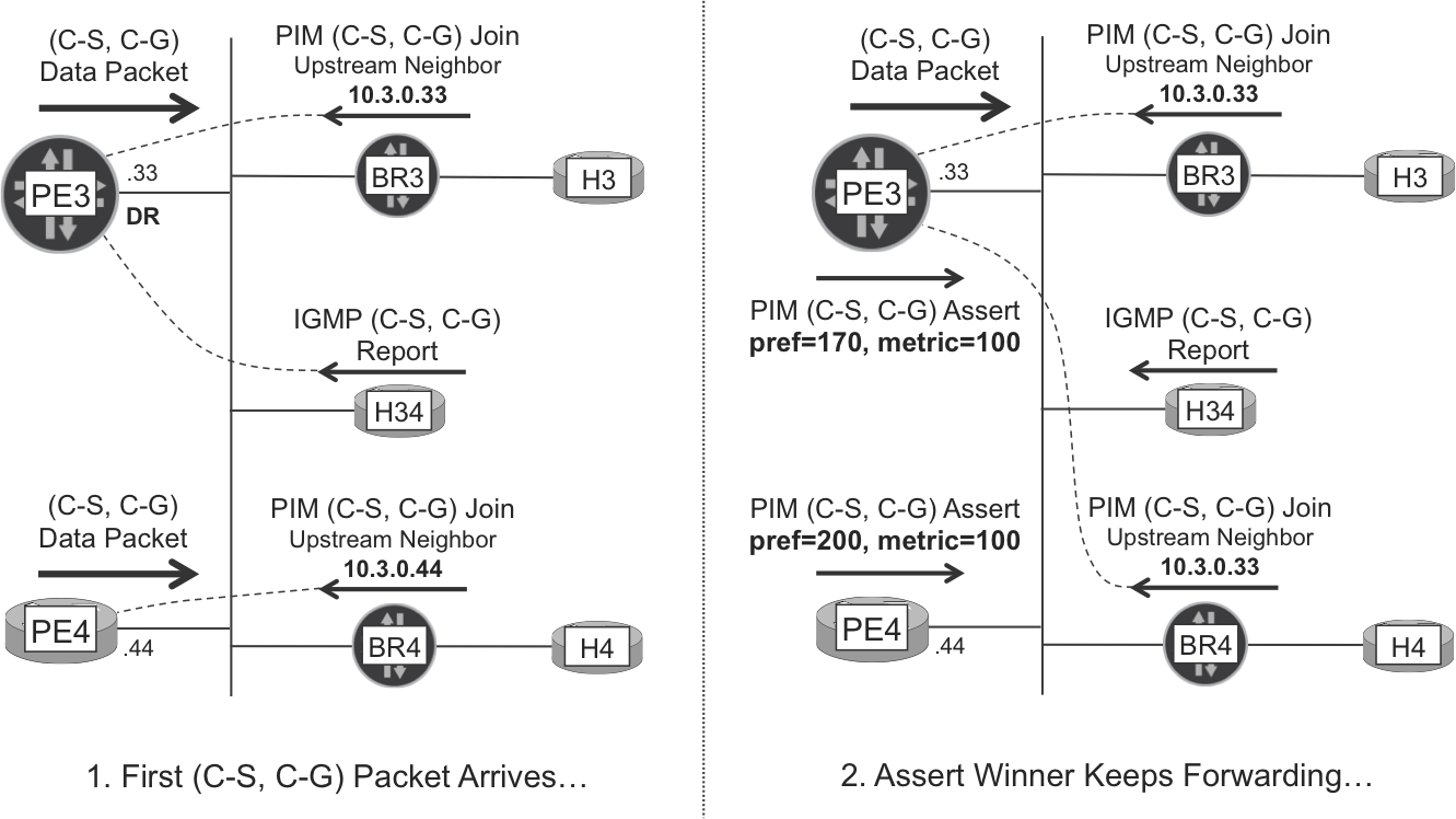
Figure 4-4. C-Multicast—egress PE redundancy and C-PIM Assert
Initially, both PE3 and PE4 are ready to forward the (10.1.1.10, 232.1.1.1) traffic to VLAN 1034. Here is why:
-
PE3 is the DR and is processing the IGMP Reports from H34.
-
PE3 is the Upstream Neighbor of a PIM (10.1.1.10, 232.1.1.1) Join sent by BR3, because BR3 only has an eBGP session with PE3.
-
PE4 is the Upstream Neighbor of a PIM (10.1.1.10, 232.1.1.1) Join sent by BR4, because BR4 only has an eBGP session with PE4.
When H1 sends the first C-Multicast packet to 232.1.1.1, both PE3 and PE4 forward it to VLAN 1034. This causes C-Multicast packet duplication in VLAN 1034, which you can verify in the first set of ping replies.
Example 4-35. mLDP P2MP LSP forwarding at a transit PE—P2 (IOS XR)
1     RP/0/0/CPU0:H# ping vrf H1 232.1.1.1 source 10.1.1.10 count 1
2     Reply to request 0 from 10.1.11.11, 1 ms
3     Reply to request 0 from 10.1.22.22, 9 ms
4     Reply to request 0 from 10.2.33.33, 9 ms
5     Reply to request 0 from 10.2.44.44, 9 ms
6     Reply to request 0 from 10.2.3.30, 9 ms
7     Reply to request 0 from 10.2.0.34, 9 ms
8     Reply to request 0 from 10.2.4.40, 9 ms
9     Reply to request 0 from 10.2.3.30, 19 ms
10    Reply to request 0 from 10.2.0.34, 19 ms
11    Reply to request 0 from 10.2.4.40, 19 ms
ICMP echo request #0 receives duplicate replies from H3, H34, and H4. From a service perspective, this is strongly undesirable. For most multicast applications, receiving a duplicate or multiplied copy of the original data stream can be as bad as not receiving it at all. For that reason, when PE3 and PE4 detect this packet duplication, they start a competition called PIM Assert, based on their route to the 10.1.1.10 multicast source.
Example 4-36. Egress PE redundancy—Unicast Route to the C-Source
1     juniper@PE3> show route active-path 10.1.1.10
2
3     inet.0: 44 destinations, 53 routes (44 active, 0 holddown, 0 hidden)
4
5     10.1.1.0/24  *[BGP/170] 1d 12:04:09, MED 100, localpref 100,
6                   from 172.16.0.201, AS path: 65001 I [...]
7                         > to 10.0.0.8 via ge-2/0/1.0, Push 300368
8
9     RP/0/0/CPU0:PE4#show route 10.1.1.10
10
11    Routing entry for 10.1.1.0/24
12      Known via "bgp 65000", distance 200, metric 100
13      Tag 65001, type internal
14      Installed Jan  6 06:11:52.147 for 15:19:12
15      Routing Descriptor Blocks
16        172.16.0.11, from 172.16.0.201
17          Route metric is 100
18      No advertising protos.
Although the MED attribute of the route is 100 in both cases, the default administrative distance of the BGP protocol is 170 on PE3 (line 5, Junos), as opposed to 200 on PE4 (line 12, IOS XR). The lowest administrative distance wins, so PE3 becomes the C-PIM (10.1.1.10, 232.1.1.1) Assert winner. At this point, PE4 stops injecting the flow on VLAN 1034. Also, because PIM Assert packets are sent to the 224.0.0.13 address, BR4 sees the Assert competition and redirects its PIM (C-S, C-G) Join Upstream Neighbor to PE3. Overall, the packet duplication in VLAN 1034 is fixed and PE3 becomes the single forwarder.
Note
There is no assert in VLAN 1044. So the fact that PE3 is the Assert winner in VLAN 1034 does not prevent PE4 from forwarding the packets to H44.
As you would expect with PIM, Assert packets are refreshed periodically. In other words, Assert, like Join/Prune, has soft state. Some minutes after the C-Source stops sending traffic, Assert times-out and the initial condition resumes (the F flag appears for VLAN 1034 in Example 4-34). So, even in a model with PIM SSM, there are scenarios in which the signaling of the multicast tree is data driven.
Ingress PE redundancy
Now, suppose that an active C-Multicast source is multihomed to PE1 and PE2, and that this source is sending traffic to (C-S, C-G). Now, both H33 and H44 send an IGMP Report subscribing to that flow. How is the P2MP LSP signaled? There are two cases:
-
Both PE3 and PE4 choose the same Upstream PE (either PE1 or PE2) as the root for the P2MP FEC. In this case, a single P2MP LSP is created, with one root and two leaves: PE3 and PE4.
-
PE3 and PE4 choose different Upstream PEs. For example, PE3 selects PE1 and PE4 selects PE2. In this case, there are two P2MP LSPs, one rooted at PE1 and the other rooted at PE2. Each of these P2MP LSPs has a single (and different) leaf.
There is no risk of data duplication in any of these cases: each egress PE signals the P2MP FEC toward a single ingress PE. This is a general advantage of Selective Trees.
mLDP In-Band and PIM ASM
As of this writing, the vendor implementations support only PIM SSM in combination with mLDP In-Band. The efforts to bring support of PIM ASM are polarized in two RFCs:
-
RFC 7438 - mLDP In-Band Signaling with Wildcards
-
RFC 7442 - Carrying PIM-SM in ASM Mode Trees over mLDP
Other Internet Multicast over MPLS Flavors
There are some additional Global Internet Multicast (S1) flavors. Here is a non-exhaustive list.
Static RSVP-TE P2MP LSPs
There is one more interoperable model to signal and transport Internet Multicast between Junos and IOS XR PEs. In Cisco documentation, it is called Global P2MP-TE. In the terms of Table 4-1, it is S1, A0, C0, E3, T3, Y3.
It relies on using static routes to place IP Multicast traffic into RSVP-TE P2MP LSPs. The network administrator manually configures the leaves of each LSP. Although you can successfully apply this model to relatively static environments such as traditional IPTV, it is not particularly appealing for the purposes of this book.
BGP Internet Multicast
Junos supports one type of routing instance called mpls-internet-multicast, which applies BGP Multicast VPN techniques to the signaling and transport of Internet Multicast traffic. In the terms of Table 4-1, it is S1, A3, C3, [E1, E2, E3], [T0, T1, T2, T3, T4], [Y1, Y2, Y3, Y4]. Not all the combinations are supported, though.
Although IOS XR does not implement this approach, you can configure the IOS XR PEs with Internet VRFs running BGP Multicast VPN. That being said, from an interoperability perspective it is more interesting to focus on the genuine BGP Multicast VPN, with VRFs on both PE types (Junos and IOS XR). Let’s go for it in Chapter 5!
Get MPLS in the SDN Era now with the O’Reilly learning platform.
O’Reilly members experience books, live events, courses curated by job role, and more from O’Reilly and nearly 200 top publishers.

