Modeling, Estimation and Optimal Filtration in Signal Processing

Appendix B

Subspace Decomposition for Spectral Analysis

Let us consider the case of a random stationary process y(k) defined as a sum of M complex exponentials of the normalized angular frequency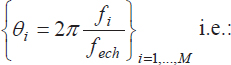

with A_i = |A_i| exp(jφ_i) where the phases φ_i are uniformly distributed over the range [0.2π] and independent of each other. Process b(k) is a zero-mean stationary white Gaussian noise with a variance σ². The autocorrelation of y(k) is thus:

where φ_i denotes the variance of A_i.

Let us now concatenate p+1 consecutive samples of the process in a vector and define the corresponding autocorrelation matrix as follows:

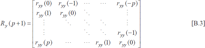
Defining matrix _i as follows;

and combining equations [B.2], [B.3] and [B.4], we can alternatively express the process vector autocorrelation matrix by carrying out an eigenvalue decomposition as follows:

Using the eigenvalues λ_i of the process vector autocorrelation matrix and arranging ...