Chapter 4. Mining Google+: Computing Document Similarity, Extracting Collocations, and More
This chapter introduces some fundamental concepts from text mining[13] and is somewhat of an inflection point in this book. Whereas we started the book with basic frequency analyses of Twitter data and gradually worked up to more sophisticated clustering analyses of messier data from LinkedIn profiles, this chapter begins munging and making sense of textual information in documents by introducing information retrieval (IR) theory fundamentals such as TF-IDF, cosine similarity, and collocation detection. Accordingly, its content is a bit more complex than that of the chapters before it, and it may be helpful to have worked through those chapters before picking up here.
Google+ initially serves as our primary source of data for this chapter because it’s inherently social, features content that’s often expressed as longer-form notes that resemble blog entries, and is now an established staple in the social web. It’s not hard to make a case that Google+ activities (notes) fill a niche somewhere between Twitter and blogs. The concepts from previous chapters could equally be applied to the data behind Google+’s diverse and powerful API, although we’ll opt to leave regurgitations of those examples (mostly) as exercises for the motivated reader.
Wherever possible we won’t reinvent the wheel and implement analysis tools from scratch, but we will take a couple of “deep dives” when particularly foundational topics come up that are essential to an understanding of text mining. The Natural Language Toolkit (NLTK) is a powerful technology that you may recall from Chapter 3; it provides many of the tools we’ll use in this chapter. Its rich suites of APIs can be a bit overwhelming at first, but don’t worry: while text analytics is an incredibly diverse and complex field of study, there are lots of powerful fundamentals that can take you a long way without too significant of an investment. This chapter and the chapters after it aim to hone in on those fundamentals. (A full-blown introduction to NLTK is outside the scope of this book, but you can review the full text of Natural Language Processing with Python: Analyzing Text with the Natural Language Toolkit [O’Reilly] at the NLTK website.)
Note
Always get the latest bug-fixed source code for this chapter (and every other chapter) online at http://bit.ly/MiningTheSocialWeb2E. Be sure to also take advantage of this book’s virtual machine experience, as described in Appendix A, to maximize your enjoyment of the sample code.
Overview
This chapter uses Google+ to begin our journey in analyzing human language data. In this chapter you’ll learn about:
The Google+ API and making API requests
TF-IDF (Term Frequency–Inverse Document Frequency), a fundamental technique for analyzing words in documents
How to apply NLTK to the problem of understanding human language
How to apply cosine similarity to common problems such as querying documents by keyword
How to extract meaningful phrases from human language data by detecting collocation patterns
Exploring the Google+ API
Anyone with a Gmail account can trivially create a Google+ account and start collaborating with friends. From a product standpoint, Google+ has evolved rapidly and used some of the most compelling features of existing social network platforms such as Twitter and Facebook in carving out its own set of unique capabilities. As with the other social websites featured in this book, a full overview of Google+ isn’t in scope for this chapter, but you can easily read about it (or sign up) online. The best way to learn is by creating an account and spending some time exploring. For the most part, where there’s a feature in the user interface, there’s an API that provides that feature that you can tap into. Suffice it to say that Google+ has leveraged tried-and-true features of existing social networks, such as marking content with hashtags and maintaining a profile according to customizable privacy settings, with additional novelties such as a fresh take on content sharing called circles, video chats called hangouts, and extensive integration with other Google services such as Gmail contacts. In Google+ API parlance, social interactions are framed in terms of people, activities, comments, and moments.
The API documentation that’s available online is always the definitive source of guidance, but a brief overview may be helpful to get you thinking about how Google+ compares to another platform such as Twitter or Facebook:
- People
People are Google+ users. Programmatically, you’ll either discover users by using the search API, look them up by a personalized URL if they’re a celebrity type,[14] or strip their Google+ IDs out of the URLs that appear in your web browser and use them for exploring their profiles. Later in this chapter, we’ll use the search API to find users on Google+.
- Activities
Activities are the things that people do on Google+. An activity is essentially a note and can be as long or short as the author likes: it can be as long as a blog post, or it can be devoid of any real textual meaning (e.g., just used to share links or multimedia content). Given a Google+ user, you can easily retrieve a list of that person’s activities, and we’ll do that later in this chapter. Like a tweet, an activity contains a lot of fascinating metadata , such as the number of times the activity has been reshared.
- Comments
Leaving comments is the way Google+ users interact with one another. Simple statistical analysis of comments on Google+ could be very interesting and potentially reveal a lot of insights into a person’s social circles or the virality of content. For example, which other Google+ users most frequently comment on activities? Which activities have the highest numbers of comments (and why)?
- Moments
Moments are a relatively recent addition to Google+ and represent a way of capturing interactions between a user and a Google+ application. Moments are similar to Facebook’s social graph stories in that they are designed to capture and create opportunities for user interaction with an application that can be displayed on a timeline. For example, if you were to make a purchase in an application, upload a photo, or watch a YouTube video, it could be captured as a moment (something you did in time) and displayed in a history of your actions or shared with friends in an activity stream by the application.
For the purposes of this chapter, we’ll be focusing on harvesting and analyzing Google+ activity data that is textual and intended to convey the same kind of meaning that you might encounter in a tweet, blog post, or Facebook status update. In other words, we’ll be trying to analyze human language data. If you haven’t signed up for Google+ yet, it’s worth taking the time to do so, as well as spending a few moments to familiarize yourself with a Google+ profile. One of the easiest ways to find specific users on Google+ is to just search for them at http://plus.google.com, and explore the platform from there.
As you explore Google+, bear in mind that it has a unique set of capabilities and is a little awkward to compare directly to other social web properties. If you’re expecting it to be a straightforward comparison, you might find yourself a bit surprised. It’s similar to Twitter in that it provides a “following” model where you can add individuals to one of your Google+ circles and keep up with their happenings without any approval on their part, but the Google+ platform also offers rich integration with other Google web properties, sports a powerful feature for videoconferencing (hangouts), and has an API similar to Facebook’s in the way that users share content and interact. Without further ado, let’s get busy exploring the API and work toward mining some data.
Making Google+ API Requests
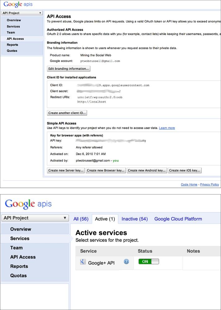
From a software development standpoint, Google+ leverages OAuth like the rest of the social web to enable an application that you’ll build to access data on a user’s behalf, so you’ll need to register an application to get appropriate credentials for accessing the Google+ platform. The Google API Console provides a means of registering an application (called a project in the Google API Console) to get OAuth credentials but also exposes an API key that you can use for “simple API access.” This API key is what we’ll use in this chapter to programmatically access the Google+ platform and just about every other Google service.
Once you’ve created an application, you’ll also need to specifically enable it to use Google+ as a separate step. Figure 4-1 provides a screenshot of the Google+ API Console as well as a view that demonstrates what it looks like when you have enabled your application for Google+ API access.
You can install a Python package called google-api-python-client for accessing
Google’s API via pip install
google-api-python-client. This is one of the standard Python-based options for accessing
Google+ data. The online documentation for google-api-python-client is marginally
helpful in familiarizing yourself with the capabilities of what it
offers, but in general, you’ll just be plugging parameters from the
official Google+ API documents into some predictable access patterns
with the Python package. Once you’ve walked through a couple of
exercises, it’s a relatively straightforward process.
Note
Don’t forget that pydoc can
be helpful for gathering clues about a package, class, or method in
a terminal as you are learning it. The help function in a standard Python
interpreter is also useful. Recall that appending ? to a method name in IPython is a
shortcut for displaying its docstring.
As an initial exercise, let’s consider the problem of locating a person on Google+. Like any other social web API, the Google+ API offers a means of searching, and in particular we’ll be interested in the People: search API. Example 4-1 illustrates how to search for a person with the Google+ API. Since Tim O’Reilly is a well-known personality with an active and compelling Google+ account, let’s look him up.
The basic pattern that you’ll repeatedly use with the Python
client is to create an instance of a service that’s parameterized for
Google+ access with your API key that you can then instantiate for
particular platform services. Here, we create a connection to
the People API by invoking service.people() and then chaining on some
additional API operations deduced from reviewing the API documentation
online. In a moment we’ll query for activity data, and you’ll see that the same
basic pattern holds.
importhttplib2importjsonimportapiclient.discovery# pip install google-api-python-client# XXX: Enter any person's nameQ="Tim O'Reilly"# XXX: Enter in your API key from https://code.google.com/apis/consoleAPI_KEY=''service=apiclient.discovery.build('plus','v1',http=httplib2.Http(),developerKey=API_KEY)people_feed=service.people().search(query=Q).execute()json.dumps(people_feed['items'],indent=1)
Following are sample results for searching for Tim O’Reilly:
[{"kind":"plus#person","displayName":"Tim O'Reilly","url":"https://plus.google.com/+TimOReilly","image":{"url":"https://lh4.googleusercontent.com/-J8..."},"etag":"\"WIBkkymG3C8dXBjiaEVMpCLNTTs/wwgOCMn..."","id":"107033731246200681024","objectType":"person"},{"kind":"plus#person","displayName":"Tim O'Reilly","url":"https://plus.google.com/11566571170551...","image":{"url":"https://lh3.googleusercontent.com/-yka..."},"etag":"\"WIBkkymG3C8dXBjiaEVMpCLNTTs/0z-EwRK7..."","id":"115665711705516993369","objectType":"person"},...]
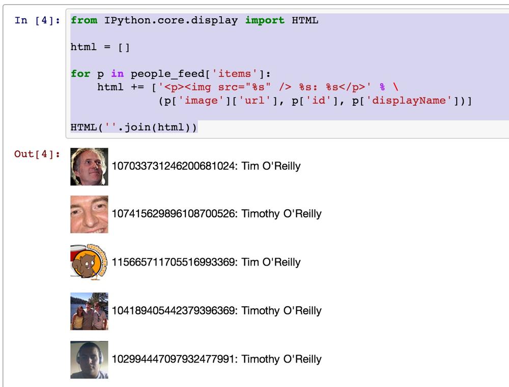
The results do indeed return a list of people named Tim O’Reilly, but how can we tell which one of these results refers to the well-known Tim O’Reilly of technology fame that we are looking for? One option would be to request profile or activity information for each of these results and try to disambiguate them manually. Another option is to render the avatars included in each of the results, which is trivial to do by rendering the avatars as images within IPython Notebook. Example 4-2 illustrates how to display avatars and the corresponding ID values for each search result by generating HTML and rendering it inline as a result in the notebook.
fromIPython.core.displayimportHTMLhtml=[]forpinpeople_feed['items']:html+=['<p><img src="%s" />%s:%s</p>'%\(p['image']['url'],p['id'],p['displayName'])]HTML(''.join(html))
Sample results are displayed in Figure 4-2 and provide the “quick fix” that we’re looking for in our search for the particular Tim O’Reilly of O’Reilly Media.
Although there’s a multiplicity of things we could do with the People API, our focus in this chapter is on an analysis of the textual content in accounts, so let’s turn our attention to the task of retrieving activities associated with this account. As you’re about to find out, Google+ activities are the linchpin of Google+ content, containing a variety of rich content associated with the account and providing logical pivots to other platform objects such as comments. To get some activities, we’ll need to tweak the design pattern we applied for searching for people, as illustrated in Example 4-3.
importhttplib2importjsonimportapiclient.discoveryUSER_ID='107033731246200681024'# Tim O'Reilly# XXX: Re-enter your API_KEY from https://code.google.com/apis/console# if not currently set# API_KEY = ''service=apiclient.discovery.build('plus','v1',http=httplib2.Http(),developerKey=API_KEY)activity_feed=service.activities().list(userId=USER_ID,collection='public',maxResults='100'# Max allowed per API).execute()json.dumps(activity_feed,indent=1)
Sample results for the first item in the results (activity_feed['items'][0]) follow and
illustrate the basic nature of a Google+ activity:
{"kind":"plus#activity","provider":{"title":"Google+"},"title":"This is the best piece about privacy that I've read in a ...","url":"https://plus.google.com/107033731246200681024/posts/78UeZ1jdRsQ","object":{"resharers":{"totalItems":191,"selfLink":"https://www.googleapis.com/plus/v1/activities/z125xvy..."},"attachments":[{"content":"Many governments (including our own, here in the US) ...","url":"http://www.zdziarski.com/blog/?p=2155","displayName":"On Expectation of Privacy | Jonathan Zdziarski's Domain","objectType":"article"}],"url":"https://plus.google.com/107033731246200681024/posts/78UeZ1jdRsQ","content":"This is the best piece about privacy that I've read ...","plusoners":{"totalItems":356,"selfLink":"https://www.googleapis.com/plus/v1/activities/z125xvyid..."},"replies":{"totalItems":48,"selfLink":"https://www.googleapis.com/plus/v1/activities/z125xvyid..."},"objectType":"note"},"updated":"2013-04-25T14:46:16.908Z","actor":{"url":"https://plus.google.com/107033731246200681024","image":{"url":"https://lh4.googleusercontent.com/-J8nmMwIhpiA/AAAAAAAAAAI/A..."},"displayName":"Tim O'Reilly","id":"107033731246200681024"},"access":{"items":[{"type":"public"}],"kind":"plus#acl","description":"Public"},"verb":"post","etag":"\"WIBkkymG3C8dXBjiaEVMpCLNTTs/d-ppAzuVZpXrW_YeLXc5ctstsCM\"","published":"2013-04-25T14:46:16.908Z","id":"z125xvyidpqjdtol423gcxizetybvpydh"}
Each activity object follows a three-tuple pattern of the form (actor, verb, object). In this post, the tuple (Tim O’Reilly, post, note) tells us that this particular item in the results is a note, which is essentially just a status update with some textual content. A closer look at the result reveals that the content is something that Tim O’Reilly feels strongly about as indicated by the title “This is the best piece about privacy that I’ve read in a long time!” and hints that the note is active as evidenced by the number of reshares and comments.
If you reviewed the output carefully, you may have noticed that
the content field for
the activity contains HTML markup, as evidenced by the HTML entity
I've that appears. In
general, you should assume that the textual data exposed as Google+
activities contains some basic markup—such as <br /> tags and escaped HTML entities
for apostrophes—so as a best practice we need to do a little bit of
additional filtering to clean it up. Example 4-4 provides an example of how to distill
plain text from the content field of a note by introducing a function
called cleanHtml. It
takes advantage of a clean_html
function provided by NLTK and another handy package for
manipulating HTML, called BeautifulSoup, that converts HTML entities back to plain text. If you haven’t
already encountered BeautifulSoup,
it’s a package that you won’t want to live without once you’ve added it
to your toolbox—it has the ability to process HTML in a reasonable way
even if it is invalid and violates standards or other reasonable
expectations (à la web data). You should install these packages via pip install nltk
beautifulsoup4 if you haven’t already.
fromnltkimportclean_htmlfromBeautifulSoupimportBeautifulStoneSoup# clean_html removes tags and# BeautifulStoneSoup converts HTML entitiesdefcleanHtml(html):ifhtml=="":return""returnBeautifulStoneSoup(clean_html(html),convertEntities=BeautifulStoneSoup.HTML_ENTITIES).contents[0]activity_feed['items'][0]['object']['content']cleanHtml(activity_feed['items'][0]['object']['content'])
The output from the note’s content, once cleansed with cleanHtml, is very clean text that can be
processed without additional concerns about noise in the content. As
we’ll learn in this chapter and follow-on chapters about text mining,
reduction of noise in text content is a critical aspect of improving
accuracy. The before and after content follows.
Here’s the raw content in activity_feed['items'][0]['object']['content']:
This is the best piece about privacy that I've read in a long time! If it doesn't change how you think about the privacy issue, I'll be surprised. It opens:<br/><br/>"Many governments (including our own, here in the US) would have its citizens believe that privacy is a switch (that is, you either reasonably expect it, or you don’t). This has been demonstrated in many legal tests, and abused in many circumstances ranging from spying on electronic mail, to drones in our airspace monitoring the movements of private citizens. But privacy doesn’t work like a switch – at least it shouldn’t for a country that recognizes that privacy is an inherent right. In fact, privacy, like other components to security, works in layers..."<br/><br/>Please read!
And here’s the content rendered after
cleansing with cleanHtml(activity_feed['items'][0]['object']['content']):
This is the best piece about privacy that I've read in a long time!  If it
doesn't change how you think about the privacy issue, I'll be surprised.  It
opens: "Many governments (including our own, here in the US) would have its
citizens believe that privacy is a switch (that is, you either reasonably expect it,
or you don’t). This has been demonstrated in many legal tests, and abused
in many circumstances ranging from spying on electronic mail, to drones in our
airspace monitoring the movements of private citizens. But privacy doesn’t work like
a switch – at least it shouldn’t for a country that recognizes that privacy is an
inherent right. In fact, privacy, like other components to security, works in
layers..." Please read!
The ability to query out clean text from Google+ is the basis for the remainder of the text mining exercises in this chapter, but one additional consideration that you may find useful before we focus our attention elsewhere is a pattern for fetching multiple pages of content.
Whereas the previous example fetched 100 activities, the maximum number of results for a query, it may be the case that you’ll want to iterate over an activities feed and retrieve more than the maximum number of activities per page. The pattern for pagination is outlined in the HTTP API Overview, and the Python client wrapper takes care of most of the hassle.
Example 4-5 shows how to fetch multiple pages of activities and distill the text from them if they are notes and have meaningful content.
importosimporthttplib2importjsonimportapiclient.discoveryfromBeautifulSoupimportBeautifulStoneSoupfromnltkimportclean_htmlUSER_ID='107033731246200681024'# Tim O'Reilly# XXX: Re-enter your API_KEY from https://code.google.com/apis/console# if not currently set# API_KEY = ''MAX_RESULTS=200# Will require multiple requestsdefcleanHtml(html):ifhtml=="":return""returnBeautifulStoneSoup(clean_html(html),convertEntities=BeautifulStoneSoup.HTML_ENTITIES).contents[0]service=apiclient.discovery.build('plus','v1',http=httplib2.Http(),developerKey=API_KEY)activity_feed=service.activities().list(userId=USER_ID,collection='public',maxResults='100'# Max allowed per request)activity_results=[]whileactivity_feed!=Noneandlen(activity_results)<MAX_RESULTS:activities=activity_feed.execute()if'items'inactivities:foractivityinactivities['items']:ifactivity['object']['objectType']=='note'and\activity['object']['content']!='':activity['title']=cleanHtml(activity['title'])activity['object']['content']=cleanHtml(activity['object']['content'])activity_results+=[activity]# list_next requires the previous request and response objectsactivity_feed=service.activities().list_next(activity_feed,activities)# Write the output to a file for conveniencef=open(os.path.join('resources','ch04-googleplus',USER_ID+'.json'),'w')f.write(json.dumps(activity_results,indent=1))f.close()str(len(activity_results)),"activities written to",f.name
With the know-how to explore the Google+ API and fetch some interesting human language data from activities’ content, let’s now turn our attention to the problem of analyzing the content.
A Whiz-Bang Introduction to TF-IDF
Although rigorous approaches to natural language processing (NLP) that include such things as sentence segmentation, tokenization, word chunking, and entity detection are necessary in order to achieve the deepest possible understanding of textual data, it’s helpful to first introduce some fundamentals from information retrieval theory. The remainder of this chapter introduces some of its more foundational aspects, including TF-IDF, the cosine similarity metric, and some of the theory behind collocation detection. Chapter 5 provides a deeper discussion of NLP as a logical continuation of this discussion.
Note
If you want to dig deeper into IR theory, the full text of Christopher Manning, Prabhakar Raghavan, and Hinrich Schütze’s Introduction to Information Retrieval (Cambridge University Press) is available online and provides more information than you could (probably) ever want to know about the field.
Information retrieval is an extensive field with many specialties. This discussion narrows in on TF-IDF, one of the most fundamental techniques for retrieving relevant documents from a corpus (collection). TF-IDF stands for term frequency-inverse document frequency and can be used to query a corpus by calculating normalized scores that express the relative importance of terms in the documents.
Mathematically, TF-IDF is expressed as the product of the term frequency and the inverse document frequency, tf_idf = tf*idf, where the term tf represents the importance of a term in a specific document, and idf represents the importance of a term relative to the entire corpus. Multiplying these terms together produces a score that accounts for both factors and has been an integral part of every major search engine at some point in its existence. To get a more intuitive idea of how TF-IDF works, let’s walk through each of the calculations involved in computing the overall score.
Term Frequency
For simplicity in illustration, suppose you have a corpus containing three sample documents and terms are calculated by simply breaking on whitespace, as illustrated in Example 4-6 as ordinary Python code.
corpus={'a':"Mr. Green killed Colonel Mustard in the study with the candlestick.\Mr. Green is not a very nice fellow.",'b':"Professor Plum has a green plant in his study.",'c':"Miss Scarlett watered Professor Plum's green plant while he was away\from his office last week."}terms={'a':[i.lower()foriincorpus['a'].split()],'b':[i.lower()foriincorpus['b'].split()],'c':[i.lower()foriincorpus['c'].split()]}
A term’s frequency could simply be represented as the number of
times it occurs in the text, but it is more commonly the case that you
normalize it by taking into account the total number of terms in the
text, so that the overall score accounts for document length relative to
a term’s frequency. For example, “green” (once normalized to lowercase) occurs twice in
corpus['a'] and only once in corpus['b'], so
corpus['a'] would produce a higher score if frequency were
the only scoring criterion. However, if you normalize for document
length, corpus['b'] would have a slightly higher term
frequency score for “green” (1/9) than corpus['a'] (2/19),
because corpus['b'] is shorter than
corpus['a']—even though “green” occurs more frequently in
corpus['a']. A common technique for scoring a compound
query such as “Mr. Green” is to sum the term frequency scores for each
of the query terms in each document, and return the documents ranked by
the summed term frequency score.
Let’s illustrate how term frequency works by querying our sample corpus for “Mr. Green,” which would produce the normalized scores reported in Table 4-1 for each document.
| Document | tf(mr.) | tf(green) | Sum |
corpus['a'] | 2/19 | 2/19 | 4/19 (0.2105) |
corpus['b'] | 0 | 1/9 | 1/9 (0.1111) |
corpus['c'] | 0 | 1/16 | 1/16 (0.0625) |
For this contrived example, a cumulative term frequency scoring
scheme works out and returns corpus['a'] (the document that
we’d expect it to return), since corpus['a'] is the only one that contains
the compound token “Mr. Green.” However, a number of problems could have
emerged, because the term frequency scoring model looks at each document
as an unordered collection of words. For example, queries for “Green
Mr.” or “Green Mr. Foo” would have returned the exact same scores as the
query for “Mr. Green,” even though neither of those phrases appears in
the sample sentences. Additionally, there are a number of scenarios that
we could easily contrive to illustrate fairly poor results from the term
frequency ranking technique given that trailing punctuation is not
handled properly, and that the context around tokens of interest is not
taken into account by the calculations.
Considering term frequency alone turns out to be a common source
of problems when scoring on a document-by-document basis, because it
doesn’t account for very frequent words, called stopwords,[15] that are common across many documents. In other words, all
terms are weighted equally, regardless of their actual importance. For
example, “the green plant” contains the stopword “the,” which skews overall term frequency scores
in favor of corpus['a'] because “the” appears twice in that
document, as does “green.” In contrast, in corpus['c']
“green” and “plant” each appear only once.
Consequently, the scores would break down as shown in Table 4-2, with corpus['a'] ranked as more
relevant than corpus['c'], even though intuition might lead
you to believe that ideal query results probably shouldn’t have turned
out that way. (Fortunately, however, corpus['b'] still
ranks highest.)
Inverse Document Frequency
Toolkits such as NLTK provide lists of stopwords that can be used to filter out terms such as and, a, and the, but keep in mind that there may be terms that evade even the best stopword lists and yet still are quite common to specialized domains. Although you can certainly customize a list of stopwords with domain knowledge, the inverse document frequency metric is a calculation that provides a generic normalization metric for a corpus. It works in the general case by accounting for the appearance of common terms across a set of documents by considering the total number of documents in which a query term ever appears.
The intuition behind this metric is that it produces a higher value if a term is somewhat uncommon across the corpus than if it is common, which helps to account for the problem with stopwords we just investigated. For example, a query for “green” in the corpus of sample documents should return a lower inverse document frequency score than a query for “candlestick,” because “green” appears in every document while “candlestick” appears in only one. Mathematically, the only nuance of interest for the inverse document frequency calculation is that a logarithm is used to reduce the result into a compressed range, since its usual application is in multiplying it against term frequency as a scaling factor. For reference, a logarithm function is shown in Figure 4-3; as you can see, the logarithm function grows very slowly as values for its domain increase, effectively “squashing” its input.
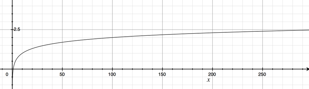
Table 4-3 provides inverse document frequency scores that correspond to the term frequency scores for in the previous section. Example 4-7 in the next section presents source code that shows how to compute these scores. In the meantime, you can notionally think of the IDF score for a term as the logarithm of a quotient that is defined by the number of documents in the corpus divided by the number of texts in the corpus that contain the term. When viewing these tables, keep in mind that whereas a term frequency score is calculated on a per-document basis, an inverse document frequency score is computed on the basis of the entire corpus. Hopefully this makes sense given that its purpose is to act as a normalizer for common words across the entire corpus.
TF-IDF
At this point, we’ve come full circle and devised a way to compute a score for a multiterm query that accounts for the frequency of terms appearing in a document, the length of the document in which any particular term appears, and the overall uniqueness of the terms across documents in the entire corpus. We can combine the concepts behind term frequency and inverse document frequency into a single score by multiplying them together, so that TF–IDF = TF*IDF. Example 4-7 is a naive implementation of this discussion that should help solidify the concepts described. Take a moment to review it, and then we’ll discuss a few sample queries.
frommathimportlog# XXX: Enter in a query term from the corpus variableQUERY_TERMS=['mr.','green']deftf(term,doc,normalize=True):doc=doc.lower().split()ifnormalize:returndoc.count(term.lower())/float(len(doc))else:returndoc.count(term.lower())/1.0defidf(term,corpus):num_texts_with_term=len([Truefortextincorpusifterm.lower()intext.lower().split()])# tf-idf calc involves multiplying against a tf value less than 0, so it's# necessary to return a value greater than 1 for consistent scoring.# (Multiplying two values less than 1 returns a value less than each of# them.)try:return1.0+log(float(len(corpus))/num_texts_with_term)exceptZeroDivisionError:return1.0deftf_idf(term,doc,corpus):returntf(term,doc)*idf(term,corpus)corpus=\{'a':'Mr. Green killed Colonel Mustard in the study with the candlestick.\Mr. Green is not a very nice fellow.','b':'Professor Plum has a green plant in his study.','c':"Miss Scarlett watered Professor Plum's green plant while he was away\from his office last week."}for(k,v)insorted(corpus.items()):k,':',v# Score queries by calculating cumulative tf_idf score for each term in queryquery_scores={'a':0,'b':0,'c':0}fortermin[t.lower()fortinQUERY_TERMS]:fordocinsorted(corpus):'TF(%s):%s'%(doc,term),tf(term,corpus[doc])'IDF:%s'%(term,),idf(term,corpus.values())fordocinsorted(corpus):score=tf_idf(term,corpus[doc],corpus.values())'TF-IDF(%s):%s'%(doc,term),scorequery_scores[doc]+=score"Overall TF-IDF scores for query '%s'"%(' '.join(QUERY_TERMS),)for(doc,score)insorted(query_scores.items()):doc,score
a : Mr. Green killed Colonel Mustard in the study...
b : Professor Plum has a green plant in his study.
c : Miss Scarlett watered Professor Plum's green...

TF(a): mr. 0.105263157895
TF(b): mr. 0.0
TF(c): mr. 0.0
IDF: mr. 2.09861228867

TF-IDF(a): mr. 0.220906556702
TF-IDF(b): mr. 0.0
TF-IDF(c): mr. 0.0

TF(a): green 0.105263157895
TF(b): green 0.111111111111
TF(c): green 0.0625
IDF: green 1.0

TF-IDF(a): green 0.105263157895
TF-IDF(b): green 0.111111111111
TF-IDF(c): green 0.0625

Overall TF-IDF scores for query 'mr. green'
a 0.326169714597
b 0.111111111111
c 0.0625
Although we’re working on a trivially small scale, the calculations involved work the same for larger data sets. Table 4-4 is a consolidated adaptation of the program’s output for three sample queries that involve four distinct terms:
“green”
“mr. green”
“the green plant”
Even though the IDF calculations for terms are computed on the basis of the entire corpus, they are displayed on a per-document basis so that you can easily verify TF-IDF scores by skimming a single row and multiplying two numbers. As you work through the query results, you’ll find that it’s remarkable just how powerful TF-IDF is, given that it doesn’t account for the proximity or ordering of words in a document.
| Document | tf(mr.) | tf(green) | tf(the) | tf(plant) |
corpus['a'] | 0.1053 | 0.1053 | 0.1053 | 0 |
corpus['b'] | 0 | 0.1111 | 0 | 0.1111 |
corpus['c'] | 0 | 0.0625 | 0 | 0.0625 |
| idf(mr.) | idf(green) | idf(the) | idf(plant) | |
| 2.0986 | 1.0 | 2.099 | 1.4055 |
| tf-idf(mr.) | tf-idf(green) | tf-idf(the) | tf-idf(plant) | |
corpus['a'] | 0.1053*2.0986 = 0.2209 | 0.1053*1.0 = 0.1053 | 0.1053*2.099 = 0.2209 | 0*1.4055 = 0 |
corpus['b'] | 0*2.0986 = 0 | 0.1111*1.0 = 0.1111 | 0*2.099 = 0 | 0.1111*1.4055 = 0.1562 |
corpus['c'] | 0*2.0986 = 0 | 0.0625*1.0 = 0.0625 | 0*2.099 = 0 | 0.0625*1.4055 = 0.0878 |
The same results for each query are shown in Table 4-5, with the TF-IDF values summed on a per-document basis.
| Query | corpus['a'] | corpus['b'] | corpus['c'] |
| green | 0.1053 | 0.1111 | 0.0625 |
| Mr. Green | 0.2209 + 0.1053 = 0.3262 | 0 + 0.1111 = 0.1111 | 0 + 0.0625 = 0.0625 |
| the green plant | 0.2209 + 0.1053 + 0 = 0.3262 | 0 + 0.1111 + 0.1562 = 0.2673 | 0 + 0.0625 + 0.0878 = 0.1503 |
From a qualitative standpoint, the query results are quite
reasonable. The corpus['b'] document
is the winner for the query “green,” with corpus['a'] just
a hair behind. In this case, the deciding factor was the length of
corpus['b'] being much smaller than that of corpus['a']—the
normalized TF score tipped the results in favor of
corpus['b'] for its one occurrence of “green,” even though
“Green” appeared in corpus['a'] two times. Since “green”
appears in all three documents, the net effect of the IDF term in the
calculations was a wash.
Do note, however, that if we had returned 0.0 instead of 1.0 for “green,” as is done in some IDF implementations, the TF-IDF scores for “green” would have been 0.0 for all three documents due the effect of multiplying the TF score by zero. Depending on the particular situation, it may be better to return 0.0 for the IDF scores rather than 1.0. For example, if you had 100,000 documents and “green” appeared in all of them, you’d almost certainly consider it to be a stopword and want to remove its effects in a query entirely.
For the query “Mr. Green,” the clear and appropriate winner is the
corpus['a'] document. However, this
document also comes out on top for the query “the green plant.” A
worthwhile exercise is to consider why corpus['a'] scored highest for this query as
opposed to corpus['b'], which at
first blush might have seemed a little more obvious.
A final nuanced point to observe is that the sample implementation
provided in Example 4-7 adjusts the IDF score by
adding a value of 1.0 to the logarithm calculation, for the purposes of
illustration and because we’re dealing with a trivial document set.
Without the 1.0 adjustment in the calculation, it would be possible to
have the idf function return values
that are less than 1.0, which would result in two fractions being
multiplied in the TF-IDF calculation. Since multiplying two fractions
together results in a value smaller than either of them, this turns out
to be an easily overlooked edge case in the TF-IDF calculation. Recall
that the intuition behind the TF-IDF calculation is that we’d like to be
able to multiply two terms in a way that consistently produces larger
TF-IDF scores for more relevant queries than for less relevant
queries.
Querying Human Language Data with TF-IDF
Let’s take the theory that you just learned about in the previous section and put it to work. In this section, you’ll get officially introduced to NLTK, a powerful toolkit for processing natural language, and use it to support the analysis of human language data that we’ll fetch from Google+.
Introducing the Natural Language Toolkit
NLTK is written such that you can explore data easily and begin to form
some impressions without a lot of upfront investment. Before skipping
ahead, though, consider following
along with the interpreter session in Example 4-8 to get a
feel for some of the powerful functionality that NLTK provides right out
of the box. Since you may not have done much work with NLTK before,
don’t forget that you can use the built-in help function to get more
information whenever you need it. For example, help(nltk)
would provide documentation on the NLTK package in an interpreter
session.
Not all of the functionality from NLTK is intended for
incorporation into production software, since output is written to the
console and not capturable into a data structure such as a list. In that
regard, methods such as nltk.text.concordance are considered “demo
functionality.” Speaking of which, many of NLTK’s modules have a
demo function that you can call to get some idea of how to use the
functionality they provide, and the source code for these demos is a
great starting point for learning how to use new APIs. For example, you
could run nltk.text.demo() in the
interpreter to get some additional insight into the capabilities
provided by the nltk.text module.
Example 4-8 demonstrates some good starting points for exploring the data with sample output included as part of an interactive interpreter session, and the same commands to explore the data are included in the IPython Notebook for this chapter. Please follow along with this example and examine the outputs of each step along the way. Are you able to follow along and understand the investigative flow of the interpreter session? Take a look, and we’ll discuss some of the details after the example.
Note
The next example includes stopwords, which—as noted earlier—are words that appear frequently in text but usually relay very little information (e.g., a, an, the, and other determinants).
# Explore some of NLTK's functionality by exploring the data.# Here are some suggestions for an interactive interpreter session.importnltk# Download ancillary nltk packages if not already installednltk.download('stopwords')all_content=" ".join([a['object']['content']forainactivity_results])# Approximate bytes of textlen(all_content)tokens=all_content.split()text=nltk.Text(tokens)# Examples of the appearance of the word "open"text.concordance("open")# Frequent collocations in the text (usually meaningful phrases)text.collocations()# Frequency analysis for words of interestfdist=text.vocab()fdist["open"]fdist["source"]fdist["web"]fdist["2.0"]# Number of words in the textlen(tokens)# Number of unique words in the textlen(fdist.keys())# Common words that aren't stopwords[wforwinfdist.keys()[:100]\ifw.lower()notinnltk.corpus.stopwords.words('english')]# Long words that aren't URLs[wforwinfdist.keys()iflen(w)>15andnotw.startswith("http")]# Number of URLslen([wforwinfdist.keys()ifw.startswith("http")])# Enumerate the frequency distributionforrank,wordinenumerate(fdist):rank,word,fdist[word]
Note
The examples throughout this chapter, including the prior
example, use the split method to tokenize text.
Tokenization isn’t quite as simple as splitting on whitespace,
however, and Chapter 5 introduces more
sophisticated approaches for tokenization that work better for the
general case.
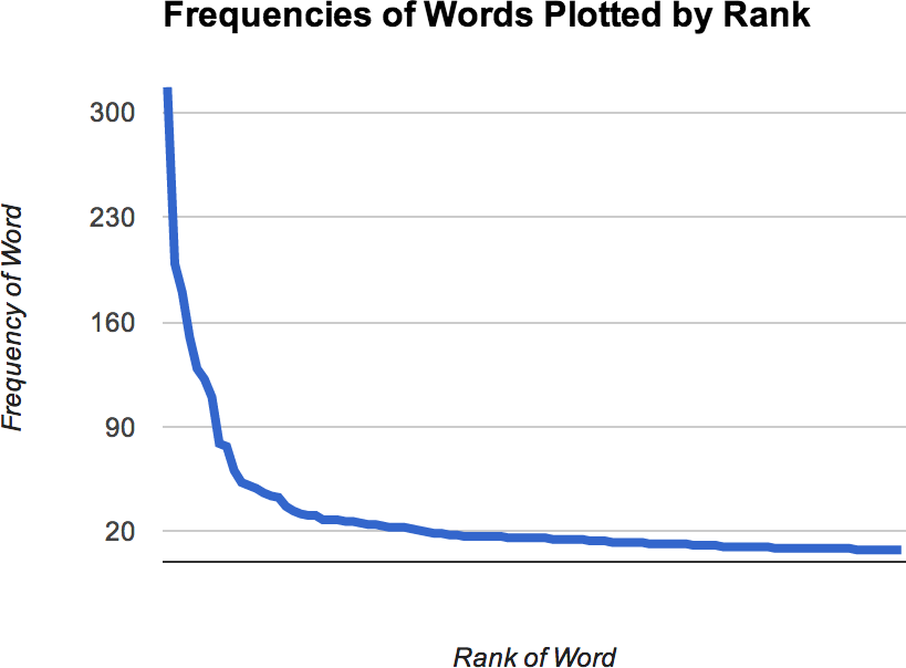
The last command in the interpreter session lists the words from the frequency distribution, sorted by frequency. Not surprisingly, stopwords like the, to, and of are the most frequently occurring, but there’s a steep decline and the distribution has a very long tail. We’re working with a small sample of text data, but this same property will hold true for any frequency analysis of natural language.
Zipf’s law, a well-known empirical law of natural language, asserts that a word’s frequency within a corpus is inversely proportional to its rank in the frequency table. What this means is that if the most frequently occurring term in a corpus accounts for N% of the total words, the second most frequently occurring term in the corpus should account for (N/2)% of the words, the third most frequent term for (N/3)% of the words, and so on. When graphed, such a distribution (even for a small sample of data) shows a curve that hugs each axis, as you can see in Figure 4-4.
Though perhaps not initially obvious, most of the area in such a distribution lies in its tail and for a corpus large enough to span a reasonable sample of a language, the tail is always quite long. If you were to plot this kind of distribution on a chart where each axis was scaled by a logarithm, the curve would approach a straight line for a representative sample size.
Zipf’s law gives you insight into what a frequency distribution for words appearing in a corpus should look like, and it provides some rules of thumb that can be useful in estimating frequency. For example, if you know that there are a million (nonunique) words in a corpus, and you assume that the most frequently used word (usually the, in English) accounts for 7% of the words,[16] you could derive the total number of logical calculations an algorithm performs if you were to consider a particular slice of the terms from the frequency distribution. Sometimes this kind of simple, back-of-the-napkin arithmetic is all that it takes to sanity-check assumptions about a long-running wall-clock time, or confirm whether certain computations on a large enough data set are even tractable.
Note
Can you graph the same kind of curve shown in Figure 4-4 for the content from a few hundred Google+ activities using the techniques introduced in this chapter combined with IPython’s plotting functionality, as introduced in Chapter 1?
Applying TF-IDF to Human Language
Let’s apply TF-IDF to the Google+ data we collected earlier and see how it works out as a tool for querying the data. NLTK provides some abstractions that we can use instead of rolling our own, so there’s actually very little to do now that you understand the underlying theory. The listing in Example 4-9 assumes you saved the working Google+ data from earlier in this chapter as a JSON file, and it allows you to pass in multiple query terms that are used to score the documents by relevance.
importjsonimportnltk# Load in human language data from wherever you've saved itDATA='resources/ch04-googleplus/107033731246200681024.json'data=json.loads(open(DATA).read())# XXX: Provide your own query terms hereQUERY_TERMS=['SOPA']activities=[activity['object']['content'].lower().split()\foractivityindata\ifactivity['object']['content']!=""]# TextCollection provides tf, idf, and tf_idf abstractions so# that we don't have to maintain/compute them ourselvestc=nltk.TextCollection(activities)relevant_activities=[]foridxinrange(len(activities)):score=0fortermin[t.lower()fortinQUERY_TERMS]:score+=tc.tf_idf(term,activities[idx])ifscore>0:relevant_activities.append({'score':score,'title':data[idx]['title'],'url':data[idx]['url']})# Sort by score and display resultsrelevant_activities=sorted(relevant_activities,key=lambdap:p['score'],reverse=True)foractivityinrelevant_activities:activity['title']'\tLink:%s'%(activity['url'],)'\tScore:%s'%(activity['score'],)
Sample query results for “SOPA,” a controversial piece of proposed legislation, on Tim O’Reilly’s Google+ data are as follows:
I think the key point of this piece by +Mike Loukides, that PIPA and SOPA provide
a "right of ext...
    Link: https://plus.google.com/107033731246200681024/posts/ULi4RYpvQGT
    Score: 0.0805961208217

Learn to Be a Better Activist During the SOPA Blackouts +Clay Johnson has put
together an awesome...
    Link: https://plus.google.com/107033731246200681024/posts/hrC5aj7gS6v
    Score: 0.0255051015259

SOPA and PIPA are bad industrial policy There are many arguments against SOPA
and PIPA that are b...
    Link: https://plus.google.com/107033731246200681024/posts/LZs8TekXK2T
    Score: 0.0227351539694

Further thoughts on SOPA, and why Congress shouldn't listen to lobbyists
Colleen Taylor of GigaOM...
    Link: https://plus.google.com/107033731246200681024/posts/5Xd3VjFR8gx
    Score: 0.0112879721039

...
Given a search term, being able to zero in on three Google+
content items ranked by relevance is of tremendous benefit when
analyzing unstructured text data. Try out some other queries and
qualitatively review the results to see for yourself how well the TF-IDF
metric works, keeping in mind that the absolute values of the scores
aren’t really important—it’s the
ability to find and sort documents by relevance that matters. Then,
begin to ponder the countless ways that you could tune or augment this
metric to be even more effective. One obvious improvement that’s left as
an exercise for the reader is to stem verbs so that variations in
elements such as tense and grammatical role resolve to the same stem and
can be more accurately accounted for in similarity calculations. The
nltk.stem module provides easy-to-use implementations for
several common stemming algorithms.
Now let’s take our new tools and apply them to the foundational problem of finding similar documents. After all, once you’ve zeroed in on a document of interest, the next natural step is to discover other content that might be of interest.
Finding Similar Documents
Once you’ve queried and discovered documents of interest, one of the next things you might want to do is find similar documents. Whereas TF-IDF can provide the means to narrow down a corpus based on search terms, cosine similarity is one of the most common techniques for comparing documents to one another, which is the essence of finding a similar document. An understanding of cosine similarity requires a brief introduction to vector space models, which is the topic of the next section.
The theory behind vector space models and cosine similarity
While it has been emphasized that TF-IDF models documents as unordered collections of words, another convenient way to model documents is with a model called a vector space. The basic theory behind a vector space model is that you have a large multidimensional space that contains one vector for each document, and the distance between any two vectors indicates the similarity of the corresponding documents. One of the most beautiful things about vector space models is that you can also represent a query as a vector and discover the most relevant documents for the query by finding the document vectors with the shortest distance to the query vector.
Although it’s virtually impossible to do this subject justice in a short section, it’s important to have a basic understanding of vector space models if you have any interest at all in text mining or the IR field. If you’re not interested in the background theory and want to jump straight into implementation details on good faith, feel free to skip ahead to the next section.
Warning
This section assumes a basic understanding of trigonometry. If your trigonometry skills are a little rusty, consider this section a great opportunity to brush up on high school math. If you’re not feeling up to it, just skim this section and rest assured that there is some mathematical rigor that backs the similarity computation we’ll be employing to find similar documents.
First, it might be helpful to clarify exactly what is meant by the term vector, since there are so many subtle variations associated with it across various fields of study. Generally speaking, a vector is a list of numbers that expresses both a direction relative to an origin and a magnitude, which is the distance from that origin. A vector can naturally be represented as a line segment drawn between the origin and a point in an N-dimensional space.
To illustrate, imagine a document that is defined by only two terms (“Open” and “Web”), with a corresponding vector of (0.45, 0.67), where the values in the vector are values such as TF-IDF scores for the terms. In a vector space, this document could be represented in two dimensions by a line segment extending from the origin at (0, 0) to the point at (0.45, 0.67). In reference to an x/y plane, the x-axis would represent “Open,” the y-axis would represent “Web,” and the vector from (0, 0) to (0.45, 0.67) would represent the document in question. Nontrivial documents generally contain hundreds of terms at a minimum, but the same fundamentals apply for modeling documents in these higher-dimensional spaces; it’s just harder to visualize.
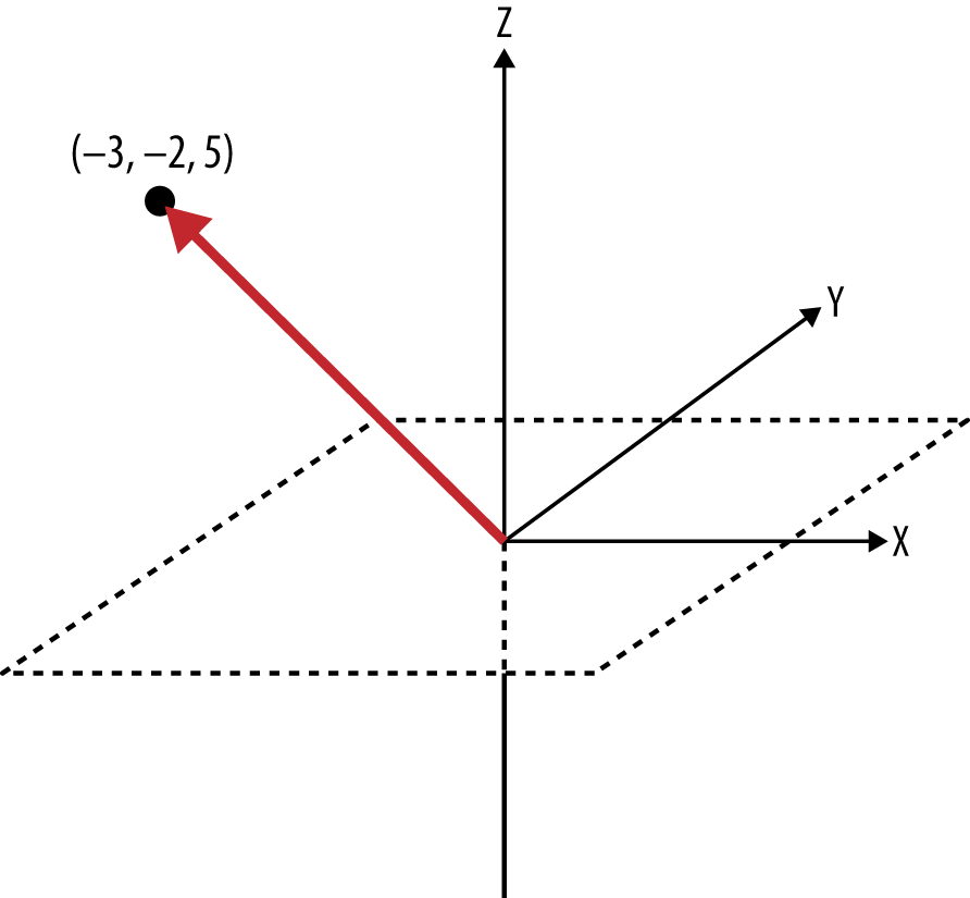
Try making the transition from visualizing a document represented by a vector with two components to a document represented by three dimensions, such as (“Open,” “Web,” and “Government”). Then consider taking a leap of faith and accepting that although it’s hard to visualize, it is still possible to have a vector represent additional dimensions that you can’t easily sketch out or see. If you’re able to do that, you should have no problem believing that the same vector operations that can be applied to a 2-dimensional space can be applied equally well to a 10-dimensional space or a 367-dimensional space. Figure 4-5 shows an example vector in 3-dimensional space.
Given that it’s possible to model documents as term-centric vectors, with each term in the document represented by its corresponding TF-IDF score, the task is to determine what metric best represents the similarity between two documents. As it turns out, the cosine of the angle between any two vectors is a valid metric for comparing them and is known as the cosine similarity of the vectors. Although it’s perhaps not yet intuitive, years of scientific research have demonstrated that computing the cosine similarity of documents represented as term vectors is a very effective metric. (It does suffer from many of the same problems as TF-IDF, though; see Closing Remarks for a brief synopsis.) Building up a rigorous proof of the details behind the cosine similarity metric would be beyond the scope of this book, but the gist is that the cosine of the angle between any two vectors indicates the similarity between them and is equivalent to the dot product of their unit vectors.
Intuitively, it might be helpful to consider that the closer two vectors are to one another, the smaller the angle between them will be, and thus the larger the cosine of the angle between them will be. Two identical vectors would have an angle of 0 degrees and a similarity metric of 1.0, while two vectors that are orthogonal to one another would have an angle of 90 degrees and a similarity metric of 0.0. The following sketch attempts to demonstrate:
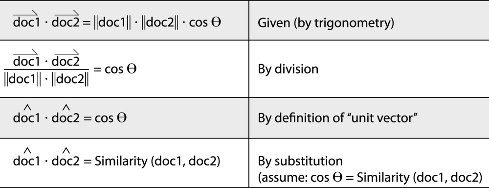
Recalling that a unit vector has a length of 1.0 (by definition), you can see that the beauty of computing document similarity with unit vectors is that they’re already normalized against what might be substantial variations in length. We’ll put all of this newly found knowledge to work in the next section.
Clustering posts with cosine similarity
One of the most important points to internalize from the previous
discussion is that to compute the similarity between two
documents, you really just need to produce a term vector for each
document and compute the dot product of the unit vectors for those
documents.
Conveniently, NLTK exposes the nltk.cluster.util.cosine_distance(v1,v2)
function for computing cosine similarity, so it really is pretty
straightforward to compare documents. As the upcoming Example 4-10 shows, all of the work involved
is in producing the appropriate term vectors; in short, it computes
term vectors for a given pair of documents by assigning TF-IDF scores
to each component in the vectors. Because the exact vocabularies of
the two documents are probably not identical, however, placeholders
with a value of 0.0 must be left in each vector for words that are
missing from the document at hand but present in the other one. The
net effect is that you end up with two vectors of identical length
with components ordered identically that can be used to perform the
vector operations.
For example, suppose document1 contained
the terms (A, B, C) and had the corresponding
vector of TF-IDF weights (0.10, 0.15, 0.12),
while document2 contained the terms (C,
D, E) with the corresponding vector of TF-IDF weights
(0.05, 0.10, 0.09). The derived vector for
document1 would be (0.10, 0.15, 0.12,
0.0, 0.0), and the derived vector for
document2 would be (0.0, 0.0, 0.05,
0.10, 0.09). Each of these vectors could be passed into
NLTK’s cosine_distance function,
which yields the cosine similarity. Internally, cosine_distance uses the numpy module to very
efficiently compute the dot product of the unit vectors, and that’s
the result. Although the code in this section reuses the TF-IDF
calculations that were introduced previously, the exact scoring
function could be any useful
metric. TF-IDF (or some variation thereof), however, is quite common
for many implementations and provides a great starting point.
Example 4-10 illustrates an approach for using cosine similarity to find the most similar document to each document in a corpus of Google+ data. It should apply equally well to any other type of human language data, such as blog posts or books.
importjsonimportnltk# Load in human language data from wherever you've saved itDATA='resources/ch04-googleplus/107033731246200681024.json'data=json.loads(open(DATA).read())# Only consider content that's ~1000+ words.data=[postforpostinjson.loads(open(DATA).read())iflen(post['object']['content'])>1000]all_posts=[post['object']['content'].lower().split()forpostindata]# Provides tf, idf, and tf_idf abstractions for scoringtc=nltk.TextCollection(all_posts)# Compute a term-document matrix such that td_matrix[doc_title][term]# returns a tf-idf score for the term in the documenttd_matrix={}foridxinrange(len(all_posts)):post=all_posts[idx]fdist=nltk.FreqDist(post)doc_title=data[idx]['title']url=data[idx]['url']td_matrix[(doc_title,url)]={}forterminfdist.iterkeys():td_matrix[(doc_title,url)][term]=tc.tf_idf(term,post)# Build vectors such that term scores are in the same positions...distances={}for(title1,url1)intd_matrix.keys():distances[(title1,url1)]={}(min_dist,most_similar)=(1.0,('',''))for(title2,url2)intd_matrix.keys():# Take care not to mutate the original data structures# since we're in a loop and need the originals multiple timesterms1=td_matrix[(title1,url1)].copy()terms2=td_matrix[(title2,url2)].copy()# Fill in "gaps" in each map so vectors of the same length can be computedforterm1interms1:ifterm1notinterms2:terms2[term1]=0forterm2interms2:ifterm2notinterms1:terms1[term2]=0# Create vectors from term mapsv1=[scorefor(term,score)insorted(terms1.items())]v2=[scorefor(term,score)insorted(terms2.items())]# Compute similarity amongst documentsdistances[(title1,url1)][(title2,url2)]=\nltk.cluster.util.cosine_distance(v1,v2)ifurl1==url2:#print distances[(title1, url1)][(title2, url2)]continueifdistances[(title1,url1)][(title2,url2)]<min_dist:(min_dist,most_similar)=(distances[(title1,url1)][(title2,url2)],(title2,url2))'''Most similar to%s(%s)\t%s(%s)\tscore%f'''%(title1,url1,most_similar[0],most_similar[1],1-min_dist)
If you’ve found this discussion of cosine similarity interesting, it might at first seem almost magical when you realize that the best part is that querying a vector space is the same operation as computing the similarity between documents, except that instead of comparing just document vectors, you compare your query vector and the document vectors. Take a moment to think about it: it’s a rather profound insight that the mathematics work out that way.
In terms of implementing a program to compute similarity across an entire corpus, however, take note that the naive approach means constructing a vector containing your query terms and comparing it to every single document in the corpus. Clearly, the approach of directly comparing a query vector to every possible document vector is not a good idea for even a corpus of modest size, and you’d need to make some good engineering decisions involving the appropriate use of indexes to achieve a scalable solution. We briefly touched upon the fundamental problem of needing a dimensionality reduction as a common staple in clustering in Chapter 3, and here we see the same concept emerge. Any time you encounter a similarity computation, you will almost imminently encounter the need for a dimensionality reduction to make the computation tractable.
Visualizing document similarity with a matrix diagram
The approach for visualizing similarity between items as introduced in this section is by using use graph-like structures, where a link between documents encodes a measure of the similarity between them. This situation presents an excellent opportunity to introduce more visualizations from D3, the state-of-the-art visualization toolkit introduced in Chapter 2. D3 is specifically designed with the interests of data scientists in mind, offers a familiar declarative syntax, and achieves a nice middle ground between high-level and low-level interfaces.
A minimal adaptation to Example 4-10 is all that’s needed to emit a collection of nodes and edges that can be used to produce visualizations similar to those in the D3 examples gallery. A nested loop can compute the similarity between the documents in our sample corpus of Google+ data from earlier in this chapter, and linkages between items may be determined based upon a simple statistical thresholding criterion.
Note
The details associated with munging the data and producing the output required to power the visualizations won’t be presented here, but the turnkey example code is provided in the IPython Notebook for this chapter.
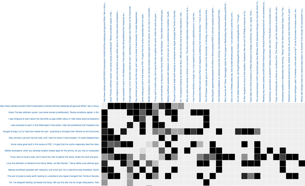
The code produces the matrix diagram in Figure 4-6. Although the text labels are not readily viewable as printed in this image, you could look at the cells in the matrix for patterns and view the labels in your browser with an interactive visualization. For example, hovering over a cell might display a tool tip with each label.
An advantage of a matrix diagram versus a graph-based layout is that there’s no potential for messy overlap between edges that represent linkages, so you avoid the proverbial “hairball” problem with your display. However, the ordering of rows and columns affects the intuition about the patterns that may be present in the matrix, so careful thought should be given to the best ordering for the rows and columns. Usually, rows and columns have additional properties that could be used to order them such that it’s easier to pinpoint patterns in the data. A recommended exercise for this chapter is to spend some time enhancing the capabilities of this matrix diagram.
Analyzing Bigrams in Human Language
As previously mentioned, one issue that is frequently overlooked in unstructured text processing is the tremendous amount of information gained when you’re able to look at more than one token at a time, because so many concepts we express are phrases and not just single words. For example, if someone were to tell you that a few of the most common terms in a post are “open,” “source,” and “government,” could you necessarily say that the text is probably about “open source,” “open government,” both, or neither? If you had a priori knowledge of the author or content, you could probably make a good guess, but if you were relying totally on a machine to try to classify a document as being about collaborative software development or transformational government, you’d need to go back to the text and somehow determine which of the other two words most frequently occurs after “open”—that is, you’d like to find the collocations that start with the token “open.”
Recall from Chapter 3 that an n-gram is just a terse way of
expressing each possible consecutive sequence of n
tokens from a text, and it provides the foundational data structure for
computing collocations. There are always (n–1)
n-grams for any value of n,
and if you were to consider all of the bigrams (two grams) for the
sequence of tokens ["Mr.", "Green", "killed",
"Colonel", "Mustard"], you’d have four possibilities: [("Mr.", "Green"), ("Green", "killed"), ("killed",
"Colonel"), ("Colonel", "Mustard")]. You’d need a larger
sample of text than just our sample sentence to determine collocations,
but assuming you had background knowledge or additional text, the next
step would be to statistically analyze the bigrams in order to determine
which of them are likely to be collocations.
n-grams are very simple yet very powerful as
a technique for clustering commonly co-occurring words. If you compute
all of the n-grams for even a small value of
n, you’re likely to discover that some interesting
patterns emerge from the text itself with no additional work required.
(Typically, bigrams and trigrams are what you’ll often see used in
practice for data mining exercises.) For example, in considering the
bigrams for a sufficiently long text, you’re likely to discover the
proper names, such as “Mr. Green” and “Colonel Mustard,” concepts such
as “open source” or “open government,” and so forth. In fact, computing
bigrams in this way produces essentially the same results as the collocations function that you ran earlier,
except that some additional statistical analysis takes
into account the use of rare words. Similar patterns emerge when you
consider frequent trigrams and n-grams for values
of n slightly larger than three. As you already
know from Example 4-8, NLTK takes care of most of the
effort in computing n-grams, discovering
collocations in a text, discovering the context in which a token has
been used, and more. Example 4-11
demonstrates.
importnltksentence="Mr. Green killed Colonel Mustard in the study with the "+\"candlestick. Mr. Green is not a very nice fellow."nltk.ngrams(sentence.split(),2)txt=nltk.Text(sentence.split())txt.collocations()
A drawback to using built-in “demo” functionality such as
nltk.Text.collocations is that
these functions don’t usually return data structures that you
can store and manipulate. Whenever
you run into such a situation, just take a look at the underlying source
code, which is usually pretty easy to learn from and adapt for your own
purposes. Example 4-12 illustrates how you
could compute the collocations and concordance indexes for a collection
of tokens and maintain control of the results.
Note
In a Python interpreter, you can usually find the source
directory for a package on disk by accessing the package’s __file__ attribute. For example, try
printing out the value of nltk.__file__ to find where NLTK’s source
is at on disk. In IPython or IPython Notebook, you could use “double
question mark magic” function to preview the source code on the spot
by executing nltk??.
importjsonimportnltk# Load in human language data from wherever you've saved itDATA='resources/ch04-googleplus/107033731246200681024.json'data=json.loads(open(DATA).read())# Number of collocations to findN=25all_tokens=[tokenforactivityindatafortokeninactivity['object']['content'].lower().split()]finder=nltk.BigramCollocationFinder.from_words(all_tokens)finder.apply_freq_filter(2)finder.apply_word_filter(lambdaw:winnltk.corpus.stopwords.words('english'))scorer=nltk.metrics.BigramAssocMeasures.jaccardcollocations=finder.nbest(scorer,N)forcollocationincollocations:c=' '.join(collocation)c
In short, the implementation loosely follows NLTK’s collocations demo function. It filters out
bigrams that don’t appear more than a minimum number of times (two,
in this case) and then applies a
scoring metric to rank the results. In this instance, the scoring function is the well-known
Jaccard Index we discussed in Chapter 3, as defined by
nltk.metrics.BigramAssocMeasures.jaccard. A
contingency table is used by the BigramAssocMeasures class to rank the
co-occurrence of terms in any given bigram as compared to the
possibilities of other words that could have appeared in the bigram.
Conceptually, the Jaccard Index measures similarity of sets, and in this
case, the sample sets are specific comparisons of bigrams that appeared
in the text.
The details of how contingency tables and Jaccard values are calculated is arguably an advanced topic, but the next section, Contingency tables and scoring functions, provides an extended discussion of those details since they’re foundational to a deeper understanding of collocation detection.
In the meantime, though, let’s examine some output from Tim O’Reilly’s Google+ data that makes it pretty apparent that returning scored bigrams is immensely more powerful than returning only tokens, because of the additional context that grounds the terms in meaning:
ada lovelace
jennifer pahlka
hod lipson
pine nuts
safe, welcoming
1st floor,
5 southampton
7ha cost:
bcs, 1st
borrow 42
broadcom masters
building, 5
date: friday
disaster relief
dissolvable sugar
do-it-yourself festival,
dot com
fabric samples
finance protection
london, wc2e
maximizing shareholder
patron profiles
portable disaster
rural co
vat tickets:
Keeping in mind that no special heuristics or tactics that could have inspected the text for proper names based on Title Case were employed, it’s actually quite amazing that so many proper names and common phrases were sifted out of the data. For example, Ada Lovelace is a fairly well-known historical figure that Mr. O’Reilly is known to write about from time to time (given her affiliation with computing), and Jennifer Pahlka is popular for her “Code for America” work that Mr. O’Reilly closely follows. Hod Lipson is an accomplished robotics professor at Cornell University. Although you could have read through the content and picked those names out for yourself, it’s remarkable that a machine could do it for you as a means of bootstrapping your own more focused analysis.
There’s still a certain amount of inevitable noise in the results because we have not yet made any effort to clean punctuation from the tokens, but for the small amount of work we’ve put in, the results are really quite good. This might be the right time to mention that even if reasonably good natural language processing capabilities were employed, it might still be difficult to eliminate all the noise from the results of textual analysis. Getting comfortable with the noise and finding heuristics to control it is a good idea until you get to the point where you’re willing to make a significant investment in obtaining the perfect results that a well-educated human would be able to pick out from the text.
Hopefully, the primary observation you’re making at this point is
that with very little effort and time invested, we’ve been able to use
another basic technique to draw out some powerful meaning from some free
text data, and the results seem to be pretty representative of
what we already suspect should be true. This is encouraging,
because it suggests that applying the same technique to anyone else’s
Google+ data (or any other kind of unstructured text, for that matter)
would potentially be just as informative, giving you a quick glimpse
into key items that are being discussed. And just as importantly, while
the data in this case probably confirms a few things you may already
know about Tim O’Reilly, you may have learned a couple of new things, as
evidenced by the people who showed up at the top of the collocations
list. While it would be easy enough to use the concordance, a regular
expression, or even the Python string type’s built-in find method to find posts relevant to “ada lovelace,” let’s instead
take advantage of the code we developed in Example 4-9 and use TF-IDF to query for “ada
lovelace.” Here’s what comes back:
Ijustgotanfrom+SuwCharmanaboutAdaLovelaceDay,andthoughtI'd share it here, sinc...Link:https://plus..com/107033731246200681024/posts/1XSAkDs9b44Score:0.198150014715
And there you have it: the “ada lovelace” query leads us to some content about Ada Lovelace Day. You’ve effectively started with a nominal (if that) understanding of the text, zeroed in on some interesting topics using collocation analysis, and searched the text for one of those topics using TF-IDF. There’s no reason you couldn’t also use cosine similarity at this point to find the most similar post to the one about the lovely Ada Lovelace (or whatever it is that you’re keen to investigate).
Contingency tables and scoring functions
Note
This section dives into some of the more technical details
of how BigramCollocationFinder—the Jaccard
scoring function from Example 4-12—works.
If this is your first reading of the chapter or you’re not
interested in these details, feel free to skip this section and
come back to it later. It’s arguably an advanced topic, and you
don’t need to fully understand it to effectively employ the
techniques from this chapter.
A common data structure that’s used to compute metrics related to bigrams is the contingency table. The purpose of a contingency table is to compactly express the frequencies associated with the various possibilities for the appearance of different terms of a bigram. Take a look at the bold entries in Table 4-6, where token1 expresses the existence of token1 in the bigram, and ~token1 expresses that token1 does not exist in the bigram.
| token1 | ~token1 | ||
| token2 | frequency(token1, token2) | frequency(~token1, token2) | frequency(*, token2) |
| ~token2 | frequency(token1, ~token2) | frequency(~token1, ~token2) | |
| frequency(token1, *) | frequency(*, *) |
Although there are a few details associated with which cells are significant for which calculations, hopefully it’s not difficult to see that the four middle cells in the table express the frequencies associated with the appearance of various tokens in the bigram. The values in these cells can compute different similarity metrics that can be used to score and rank bigrams in order of likely significance, as was the case with the previously introduced Jaccard Index, which we’ll dissect in just a moment. First, however, let’s briefly discuss how the terms for the contingency table are computed.
The way that the various entries in the contingency table are computed is directly tied to which data structures you have precomputed or otherwise have available. If you assume that you have available only a frequency distribution for the various bigrams in the text, the way to calculate frequency(token1, token2) is a direct lookup, but what about frequency(~token1, token2)? With no other information available, you’d need to scan every single bigram for the appearance of token2 in the second slot and subtract frequency(token1, token2) from that value. (Take a moment to convince yourself that this is true if it isn’t obvious.)
However, if you assume that you have a frequency distribution available that counts the occurrences of each individual token in the text (the text’s unigrams) in addition to a frequency distribution of the bigrams, there’s a much less expensive shortcut you can take that involves two lookups and an arithmetic operation. Subtract the number of times that token2 appeared as a unigram from the number of times the bigram (token1, token2) appeared, and you’re left with the number of times the bigram (~token1, token2) appeared. For example, if the bigram (“mr.”, “green”) appeared three times and the unigram (“green”) appeared seven times, it must be the case that the bigram (~“mr.”, “green”) appeared four times (where ~“mr.” literally means “any token other than ‘mr.’”). In Table 4-6, the expression frequency(*, token2) represents the unigram token2 and is referred to as a marginal because it’s noted in the margin of the table as a shortcut. The value for frequency(token1, *) works the same way in helping to compute frequency(token1, ~token2), and the expression frequency(*, *) refers to any possible unigram and is equivalent to the total number of tokens in the text. Given frequency(token1, token2), frequency(token1, ~token2), and frequency(~token1, token2), the value of frequency(*, *) is necessary to calculate frequency(~token1, ~token2).
Although this discussion of contingency tables may seem somewhat tangential, it’s an important foundation for understanding different scoring functions. For example, consider the Jaccard Index as introduced back in Chapter 3. Conceptually, it expresses the similarity of two sets and is defined by:
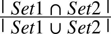
In other words, that’s the number of items in common between the two sets divided by the total number of distinct items in the combined sets. It’s worth taking a moment to ponder this simple yet effective calculation. If Set1 and Set2 were identical, the union and the intersection of the two sets would be equivalent to one another, resulting in a ratio of 1.0. If both sets were completely different, the numerator of the ratio would be 0, resulting in a value of 0.0. Then there’s everything else in between.
The Jaccard Index as applied to a particular bigram expresses the ratio between the frequency of a particular bigram and the sum of the frequencies with which any bigram containing a term in the bigram of interest appears. One interpretation of that metric might be that the higher the ratio is, the more likely it is that (token1, token2) appears in the text, and hence the more likely it is that the collocation “token1 token2” expresses a meaningful concept.
The selection of the most appropriate scoring function is
usually determined based upon knowledge about the characteristics of
the underlying data, some intuition, and sometimes a bit of luck. Most
of the association metrics defined in
nltk.metrics.associations are discussed in Chapter 5 of
Christopher Manning and Hinrich Schütze’s Foundations of Statistical Natural
Language Processing (MIT Press), which is conveniently
available online and
serves as a useful reference for the descriptions that follow.
One of the most fundamental concepts in statistics is a normal distribution. A normal distribution, often referred to as a bell curve because of its shape, is called a “normal” distribution because it is often the basis (or norm) against which other distributions are compared. It is a symmetric distribution that is perhaps the most widely used in statistics. One reason that its significance is so profound is because it provides a model for the variation that is regularly encountered in many natural phenomena in the world, ranging from physical characteristics of populations to defects in manufacturing processes and the rolling of dice.
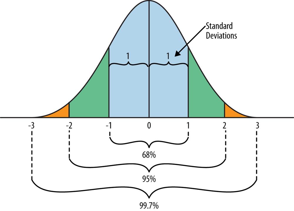
A rule of thumb that shows why the normal distribution can be so useful is the so-called 68-95-99.7 rule, a handy heuristic that can be used to answer many questions about approximately normal distributions.. For a normal distribution, it turns out that virtually all (99.7%) of the data lies within three standard deviations of the mean, 95% of it lies within two standard deviations, and 68% of it lies within one standard deviation. Thus, if you know that a distribution that explains some real-world phenomenon is approximately normal for some characteristic and its mean and standard deviation are defined, you can reason about it to answer many useful questions. Figure 4-7 illustrates the 68-95-99.7 rule.
The Khan Academy’s “Introduction to the Normal Distribution” provides an excellent 30-minute overview of the normal distribution; you might also enjoy the 10-minute segment on the central limit theorem, which is an equally profound concept in statistics in which the normal distribution emerges in a surprising (and amazing) way.
A thorough discussion of these metrics is outside the scope of this book, but the promotional chapter just mentioned provides a detailed account with in-depth examples. The Jaccard Index, Dice’s coefficient, and the likelihood ratio are good starting points if you find yourself needing to build your own collocation detector. They are described, along with some other key terms, in the list that follows:
- Raw frequency
As its name implies, raw frequency is the ratio expressing the frequency of a particular n-gram divided by the frequency of all n-grams. It is useful for examining the overall frequency of a particular collocation in a text.
- Jaccard Index
The Jaccard Index is a ratio that measures the similarity between sets. As applied to collocations, it is defined as the frequency of a particular collocation divided by the total number of collocations that contain at least one term in the collocation of interest. It is useful for determining the likelihood of whether the given terms actually form a collocation, as well as ranking the likelihood of probable collocations. Using notation consistent with previous explanations, this formulation would be mathematically defined as:

- Dice’s coefficient
Dice’s coefficient is extremely similar to the Jaccard Index. The fundamental difference is that it weights agreements among the sets twice as heavily as Jaccard. It is defined mathematically as:
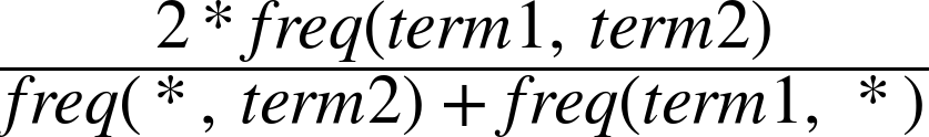
Mathematically, it can be shown fairly easily that:
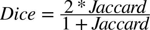
You’d likely choose to use this metric instead of the Jaccard Index when you’d like to boost the score to favor overlap between sets, which may be handy when one or more of the differences between the sets are high. The reason is that a Jaccard score inherently diminishes as the cardinality of the set differences increases in size, since the union of the set is in the denominator of the Jaccard score.
- Student’s t-score
Traditionally, Student’s t-score has been used for hypothesis testing, and as applied to n-gram analysis, t-scores can be used for testing the hypothesis of whether two terms are collocations. The statistical procedure for this calculation uses a standard distribution per the norm for t-testing. An advantage of the t-score values as opposed to raw frequencies is that a t-score takes into account the frequency of a bigram relative to its constituent components. This characteristic facilitates ranking the strengths of collocations. A criticism of the t-test is that it necessarily assumes that the underlying probability distribution for collocations is normal, which is not often the case.
- Chi-square
Like Student’s t-score, this metric is commonly used for testing independence between two variables and can be used to measure whether two tokens are collocations based upon Pearson’s chi-square test of statistical significance. Generally speaking, the differences obtained from applying the t-test and chi-square test are not substantial. The advantage of chi-square testing is that unlike t-testing, it does not assume an underlying normal distribution; for this reason, chi-square testing is more commonly used.
- Likelihood ratio
This metric is yet another approach to hypothesis testing that is used to measure the independence between terms that may form a collocation. It’s been shown to be a more appropriate approach for collocation discovery than the chi-square test in the general case, and it works well on data that includes many infrequent collocations. The particular calculations involved in computing likelihood estimates for collocations as implemented by NLTK assume a binomial distribution, where the parameters governing the distribution are calculated based upon the number of occurrences of collocations and constituent terms.
- Pointwise Mutual Information
Pointwise Mutual Information (PMI) is a measure of how much information is gained about a particular word if you also know the value of a neighboring word. To put it another way, it refers to how much one word can tell you about another. Ironically (in the context of the current discussion), the calculations involved in computing the PMI lead it to score high-frequency words lower than low-frequency words, which is the opposite of the desired effect. Therefore, it is a good measure of independence but not a good measure of dependence (i.e., it’s a less-than-ideal choice for scoring collocations). It has also been shown that sparse data is a particular stumbling block for PMI scoring, and that other techniques such as the likelihood ratio tend to outperform it.
Evaluating and determining the best method to apply in any particular situation is often as much art as science. Some problems are fairly well studied and provide a foundation that guides additional work, while some circumstances often require more novel research and experimentation. For most nontrivial problems, you’ll want to consider exploring the latest scientific literature (whether it be a textbook or a white paper from academia that you find with Google Scholar) to determine if a particular problem you are trying to solve has been well studied.
Reflections on Analyzing Human Language Data
This chapter has introduced a variety of tools and processes for analyzing human language data, and some closing reflections may be helpful in synthesizing its content:
- Context drives meaning
While TF-IDF is a powerful tool that’s easy to use, our specific implementation of it has a few important limitations that we’ve conveniently overlooked but that you should consider. One of the most fundamental is that it treats a document as a “bag of words,” which means that the order of terms in both the document and the query itself does not matter. For example, querying for “Green Mr.” would return the same results as “Mr. Green” if we didn’t implement logic to take the query term order into account or interpret the query as a phrase as opposed to a pair of independent terms. But obviously, the order in which terms appear is very important.
In performing an n-gram analysis to account for collocations and term ordering, we still face the underlying issue that TF-IDF assumes that all tokens with the same text value mean the same thing. Clearly, however, this need not be the case. A homonym is a word that has identical spellings and pronunciations to another word but whose meaning is driven entirely by context, and any homonym of your choice is a counterexample. Homonyms such as book, match, cave, and cool are a few examples that should illustrate the importance of context in determining the meaning of a word.
Cosine similarity suffers from many of the same flaws as TF-IDF. It does not take into account the context of the document or the term order from the n-gram analysis, and it assumes that terms appearing close to one another in vector space are necessarily similar, which is certainly not always the case. As with TF-IDF, the obvious counterexample is homonyms. Our particular implementation of cosine similarity also hinges on TF-IDF scoring as its means of computing the relative importance of words in documents, so the TF-IDF errors have a cascading effect.
- Human language is overloaded with context
You’ve probably noticed that there can be a lot of pesky details that have to be managed in analyzing unstructured text, and these details turn out to be pretty important for competitive implementations. For example, string comparisons are case-sensitive, so it’s important to normalize terms so that frequencies can be calculated as accurately as possible. However, blindly normalizing to lowercase can also complicate the situation since the case used in certain words and phrases can be important.
“Mr. Green” and “Web 2.0” are two examples worth considering. In the case of “Mr. Green,” maintaining the title case in “Green” could potentially be advantageous since it could provide a useful clue to a query algorithm that this term is not referring to an adjective and is likely part of a noun phrase. We’ll briefly touch on this topic again in Chapter 5 when NLP is discussed, since it’s ultimately the context in which “Green” is being used that is lost with the bag-of-words approach, whereas more advanced parsing with NLP has the potential to preserve that context.
- Parsing context from human language isn’t easy
Another consideration that’s rooted more in our particular implementation than a general characteristic of TF-IDF itself is that our use of
splitto tokenize the text may leave trailing punctuation on tokens that can affect tabulating frequencies. For example, in Example 4-6,corpus['b']ends with the token “study.”; this is not the same as the token “study” that appears incorpus['a'](the token that someone would probably be more likely to query). In this instance, the trailing period on the token affects both the TF and the IDF calculations. Something as seemingly simple as a period signaling the end of a sentence is context that our brain processes trivially, but it’s much more difficult for a machine to do this with the same level of accuracy.
Writing software to help machines better understand the context of words as they appear in human language data is a very active area of research and has tremendous potential for the future of search technology and the Web.
Closing Remarks
This chapter introduced the Google+ API and how to collect and cleanse human language data as part of an exercise in querying for a person’s Google+ activities. We then spent some time learning about a few of the fundamentals of IR theory, TF-IDF, cosine similarity, and collocations as the means of analyzing the data we collect. Eventually we worked up to the point where we were considering some of the same problems that any search engine provider has had to consider to build a successful technology product. However, even though I hope this chapter has given you some good insight into how to extract useful information from unstructured text, it’s barely scratched the surface of the most fundamental concepts, both in terms of theory and engineering considerations. Information retrieval is literally a multibillion-dollar industry, so you can only imagine the amount of combined investment that goes into both the theory and implementations that work at scale to power search engines such as Google and Bing.
Given the immense power of search providers like Google, it’s easy to forget that these foundational search techniques even exist. However, understanding them yields insight into the assumptions and limitations of the commonly accepted status quo for search, while also clearly differentiating the state-of-the-art, entity-centric techniques that are emerging. Chapter 5 introduces a fundamental paradigm shift away from some of the techniques in this chapter. There are lots of exciting opportunities for technology-driven companies that can effectively analyze human language data.
Note
The source code outlined for this chapter and all other chapters is available at GitHub in a convenient IPython Notebook format that you’re highly encouraged to try out from the comfort of your own web browser.
Recommended Exercises
Take advantage of IPython Notebook’s plotting features, introduced in Chapter 1, to graph Zipf’s curve for the tokens from a corpus.
Mine the comments feed and try to identify trends based on frequency of commenting. For example, who are the most frequent commenters across a few hundred activities for a popular Google+ user like Tim O’Reilly?
Mine Google+ activities to discover which activities are the most popular. A suitable starting point might be the number of comments and number of times a post is reshared.
Fetch the content from links that are referenced in Google+ activities and adapt the
cleanHtmlfunction from this chapter to extract the text across the web pages in a user’s activity stream for analysis. Are there any common themes in links that are shared? What are the most frequent words that appear in the text?If you’d like to try applying the techniques from this chapter to the Web (in general), you might want to check out Scrapy, an easy-to-use and mature web scraping and crawling framework that can help you to harvest web pages.
Spend some time and add interactive capabilities to the matrix diagram presented in this chapter. Can you add event handlers to automatically take you to the post when text is clicked on? Can you conceive of any meaningful ways to order the rows and columns so that it’s easier to identify patterns?
Update the code that emits the JSON that drives the matrix diagram so that it computes similarity differently and thus correlates documents differently from the default implementation.
What additional features from the text can you think of that would make computing similarity across documents more accurate?
Spend some time really digging into the theory presented in this chapter for the underlying IR concepts that were presented.
[13] This book avoids splitting hairs over exactly what differences could be implied by common phrases such as text mining, unstructured data analytics (UDA), or information retrieval, and simply treats them as essentially the same thing.
[14] Google+ only offered personalized URLs such as https://plus.google.com/+TimOReilly to well-known individuals at the outset, but is in the process of making them available to all users. Until you are either selected by Google or eligible to apply, you’ll have to continue using your more arcane URL with a numeric identifier in it (such as https://plus.google.com/107033731246200681024).
[15] Stopwords are words that appear frequently in text but usually relay little information. Common examples of stopwords are a, an, the, and other determinants.
[16] The word the accounts for 7% of the tokens in the Brown Corpus and provides a reasonable starting point for a corpus if you don’t know anything else about it.
Get Mining the Social Web, 2nd Edition now with the O’Reilly learning platform.
O’Reilly members experience books, live events, courses curated by job role, and more from O’Reilly and nearly 200 top publishers.

