Loss Models: From Data to Decisions, 4th Edition

20.3 Determining the sample size

A question asked at the beginning of this chapter remains unanswered: How many simulations are needed to achieve a desired level of accuracy? We know that any consistent estimator will be arbitrarily close to the true value with high probability as the sample size is increased. In particular, empirical estimators have this attribute. With a little effort we should be able to determine the number of simulated values needed to get us as close as we want with a specified probability. Often, the central limit theorem will help, as in the following example.

EXAMPLE 20.12

(Example 20.1 continued) Use simulation to estimate the mean, F_X(1,000), and π_0.9, the 90th percentile of the Pareto distribution with α = 3 and θ = 1,000. In each case, stop the simulations when you are 95% confident that the answer is within ±1% of the true value.

In this example we know the values. Here, μ = 500, F_X (1,000) = 0.875, and π0.9 = 1,154.43. For instructional purposes, we behave as if we do not know these values.

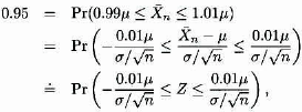
The empirical estimate of μ is . The central limit theorem tells us that for a sample of size n

where Z has the standard normal distribution. Our goal is achieved ...