Loss Models: From Data to Decisions, 4th Edition

F.2 The simplex method

The simplex method (which is not related to the simplex method from operations research) was introduced for use with maximum likelihood estimation by Nelder and Mead in 1965 [80]. An excellent reference (and the source of the particular version presented here) is Sequential Simplex Optimization by Walters, Parker, Morgan, and Deming [115].

Let x be a k x 1 vector and f(x) be the function in question. The iterative step begins with k + 1 vectors, x₁,…, x_k+1, and the corresponding functional values, f₁,…, f_k+1. At any iteration, the points will be ordered so that f₂ < ··· < f_k+1. When starting, also arrange for f₁ < f₂. Three of the points have names: x₁ is called worstpoint, x₂ is called secondworstpoint, and x_k+1 is called bestpoint. It should be noted that after the first iteration these names may not perfectly describe the points. Now identify five new points. The first one, y₁, is the center of x₂,…, x_k+1, that is, and is called midpoint, The other four points are found as follows:

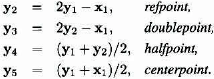
Then let g₂,…, g₅ be the corresponding functional values, that is, g_j = f(y_j) (the value at y₁ is never used). The key is to replace worstpoint (x₁) with one of these points. The five-step decision process proceeds as follows:

1. If f₂ < g₂ < f_k+1, then replace it with refpoint. ...