Learning OpenCV

Optical Flow

As already mentioned, you may often want to assess motion between two frames (or a sequence of frames) without any other prior knowledge about the content of those frames. Typically, the motion itself is what indicates that something interesting is going on. Optical flow is illustrated in Figure 10-3.

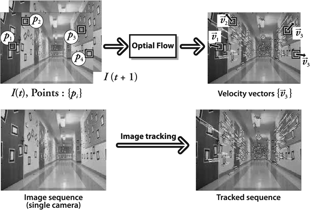
Figure 10-3. Optical flow: target features (upper left) are tracked over time and their movement is converted into velocity vectors (upper right); lower panels show a single image of the hallway (left) and flow vectors (right) as the camera moves down the hall (original images courtesy of Jean-Yves Bouguet)

We can associate some kind of velocity with each pixel in the frame or, equivalently, some displacement that represents the distance a pixel has moved between the previous frame and the current frame. Such a construction is usually referred to as a dense optical flow, which associates a velocity with every pixel in an image. The Horn-Schunck method [Horn81] attempts to compute just such a velocity field. One seemingly straightforward method—simply attempting to match windows around each pixel from one frame to the next—is also implemented in OpenCV; this is known as block matching. Both of these routines will be discussed in the "Dense Tracking Techniques" section.

In practice, calculating dense optical flow is not easy. Consider the motion of a white sheet of paper. ...