Chapter 4. Images and Large Array Types
Dynamic and Variable Storage
The next stop on our journey brings us to the large array types. Chief among these is cv::Mat, which could be considered the epicenter of the entire C++ implementation of the OpenCV library. The overwhelming majority of functions in the OpenCV library are members of the cv::Mat class, take a cv::Mat as an argument, or return cv::Mat as a return value; quite a few are or do all three.
The cv::Mat class is used to represent dense arrays of any number of dimensions. In this context, dense means that for every entry in the array, there is a data value stored in memory corresponding to that entry, even if that entry is zero. Most images, for example, are stored as dense arrays. The alternative would be a sparse array. In the case of a sparse array, only nonzero entries are typically stored. This can result in a great savings of storage space if many of the entries are in fact zero, but can be very wasteful if the array is relatively dense. A common case for using a sparse array rather than a dense array would be a histogram. For many histograms, most of the entries are zero, and storing all those zeros is not necessary. For the case of sparse arrays, OpenCV has the alternative data structure, cv::SparseMat.
Note
If you are familiar with the C interface (pre–version 2.1 implementation) of the OpenCV library, you will remember the data types IplImage and CvMat. You might also recall CvArr. In the C++ implementation, these are all gone, replaced with cv::Mat. This means no more dubious casting of void* pointers in function arguments, and in general is a tremendous enhancement in the internal cleanliness of the library.
The cv::Mat Class: N-Dimensional Dense Arrays
The cv::Mat class can be used for arrays of any number of dimensions. The data is stored in the array in what can be thought of as an n-dimensional analog of “raster scan order.” This means that in a one-dimensional array, the elements are sequential. In a two-dimensional array, the data is organized into rows, and each row appears one after the other. For three-dimensional arrays, each plane is filled out row by row, and then the planes are packed one after the other.
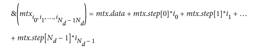
Each matrix contains a flags element signaling the contents of the array, a dims element indicating the number of dimensions, rows and cols elements indicating the number of rows and columns (these are not valid for dims>2), a data pointer to where the array data is stored, and a refcount reference counter analogous to the reference counter used by cv::Ptr<>. This latter member allows cv::Mat to behave very much like a smart pointer for the data contained in data. The memory layout in data is described by the array step[]. The data array is laid out such that the address of an element whose indices are given by ![]() is:
is:
In the simple case of a two-dimensional array, this reduces to:

The data contained in cv::Mat is not required to be simple primitives. Each element of the data in a cv::Mat can itself be either a single number or multiple numbers. In the case of multiple numbers, this is what the library refers to as a multichannel array. In fact, an n-dimensional array and an (n–1)-dimensional multichannel array are actually very similar objects, but because there are many occasions in which it is useful to think of an array as a vector-valued array, the library contains special provisions for such structures.1
One reason for this distinction is memory access. By definition, an element of an array is the part that may be vector-valued. For example, an array might be said to be a two-dimensional three-channel array of 32-bit floats; in this case, the element of the array is the three 32-bit floats with a size of 12 bytes. When laid out in memory, rows of an array may not be absolutely sequential; there may be small gaps that buffer each row before the next.2 The difference between an n-dimensional single-channel array and an (n–1)-dimensional multichannel array is that this padding will always occur at the end of full rows (i.e., the channels in an element will always be sequential).
Creating an Array
You can create an array simply by instantiating a variable of type cv::Mat. An array created in this manner has no size and no data type. You can, however, later ask it to allocate data by using a member function such as create(). One variation of create() takes as arguments a number of rows, a number of columns, and a type, and configures the array to represent a two-dimensional object. The type of an array determines what kind of elements it has. Valid types in this context specify both the fundamental type of element as well as the number of channels. All such types are defined in the library header, and have the form CV_{8U,16S,16U,32S,32F,64F}C{1,2,3}.3 For example, CV_32FC3 would imply a 32-bit floating-point three-channel array.
If you prefer, you can also specify these things when you first allocate the matrix. There are many constructors for cv::Mat, one of which takes the same arguments as create() (and an optional fourth argument with which to initialize all of the elements in your new array). For example:
cv::Mat m;

// Create data area for 3 rows and 10 columns of 3-channel 32-bit floats
m.create( 3, 10, CV_32FC3 );

// Set the values in the 1st channel to 1.0, the 2nd to 0.0, and the 3rd to 1.0
m.setTo( cv::Scalar( 1.0f, 0.0f, 1.0f ) );
is equivalent to:
cv::Mat m( 3, 10, CV_32FC3, cv::Scalar( 1.0f, 0.0f, 1.0f ) );
The Most Important Paragraph in the Book
It is critical to understand that the data in an array is not attached rigidly to the array object. The cv::Mat object is really a header for a data area, which—in principle—is an entirely separate thing. For example, it is possible to assign one matrix n to another matrix m (i.e., m=n). In this case, the data pointer inside of m will be changed to point to the same data as n. The data pointed to previously by the data element of m (if any) will be deallocated.4 At the same time, the reference counter for the data area that they both now share will be incremented. Last but not least, the members of m that characterize its data (such as rows, cols, and flags) will be updated to accurately describe the data now pointed to by data in m. This all results in a very convenient behavior, in which arrays can be assigned to one another, and the work necessary to do this takes place automatically behind the scenes to give the correct result.
Table 4-1 is a complete list of the constructors available for cv::Mat. The list appears rather unwieldy, but in fact you will use only a small fraction of these most of the time. Having said that, when you need one of the more obscure ones, you will probably be glad it is there.
| Constructor | Description |
|---|---|
cv::Mat; |
Default constructor |
cv::Mat( int rows, int cols, int type ); |
Two-dimensional arrays by type |
cv::Mat(
       int rows, int cols, int type,
       const Scalar& s
);
|
Two-dimensional arrays by type with initialization value |
cv::Mat(
       int rows, int cols, int type,
       void* data, size_t step=AUTO_STEP
);
|
Two-dimensional arrays by type with preexisting data |
cv::Mat( cv::Size sz, int type ); |
Two-dimensional arrays by type (size in sz) |
cv::Mat(
       cv::Size sz,
       int type, const Scalar& s
);
|
Two-dimensional arrays by type with initialization value (size in sz) |
cv::Mat(
       cv::Size sz, int type,
       void* data, size_t step=AUTO_STEP
 );
|
Two-dimensional arrays by type with preexisting data (size in sz) |
cv::Mat(
       int ndims, const int* sizes,
       int type
);
|
Multidimensional arrays by type |
cv::Mat(
       int ndims, const int* sizes,
       int type, const Scalar& s
 );
|
Multidimensional arrays by type with initialization value |
cv::Mat(
       int ndims, const int* sizes,
       int type, void* data,
       size_t step=AUTO_STEP
 );
|
Multidimensional arrays by type with preexisting data |
Table 4-1 lists the basic constructors for the cv::Mat object. Other than the default constructor, these fall into three basic categories: those that take a number of rows and a number of columns to create a two-dimensional array, those that use a cv::Size object to create a two-dimensional array, and those that construct n-dimensional arrays and require you to specify the number of dimensions and pass in an array of integers specifying the size of each of the dimensions.
In addition, some of these allow you to initialize the data, either by providing a cv::Scalar (in which case, the entire array will be initialized to that value), or by providing a pointer to an appropriate data block that can be used by the array. In this latter case, you are essentially just creating a header to the existing data (i.e., no data is copied; the data member is set to point to the data indicated by the data argument).
The copy constructors (Table 4-2) show how to create an array from another array. In addition to the basic copy constructor, there are three methods for constructing an array from a subregion of an existing array and one constructor that initializes the new matrix using the result of some matrix expression.
| Constructor | Description |
|---|---|
cv::Mat( const Mat& mat ); |
Copy constructor |
cv::Mat(
       const Mat& mat,
       const cv::Range& rows,
       const cv::Range& cols
 );
|
Copy constructor that copies only a subset of rows and columns |
cv::Mat(
       const Mat& mat,
       const cv::Rect& roi
);
|
Copy constructor that copies only a subset of rows and columns specified by a region of interest |
cv::Mat(
       const Mat& mat,
       const cv::Range* ranges
 );
|
Generalized region of interest copy constructor that uses an array of ranges to select from an n-dimensional array |
cv::Mat( const cv::MatExpr& expr ); |
Copy constructor that initializes m with the result of an algebraic expression of other matrices |
The subregion (also known as “region of interest”) constructors also come in three flavors: one that takes a range of rows and a range of columns (this works only on a two-dimensional matrix), one that uses a cv::Rect to specify a rectangular subregion (which also works only on a two-dimensional matrix), and a final one that takes an array of ranges. In this latter case, the number of valid ranges pointed to by the pointer argument ranges must be equal to the number of dimensions of the array mat. It is this third option that you must use if mat is a multidimensional array with ndim greater than 2.
If you are modernizing or maintaining pre–version 2.1 code that still contains the C-style data structures, you may want to create a new C++-style cv::Mat structure from an existing CvMat or IplImage structure. In this case, you have two options (Table 4-3): you can construct a header m on the existing data (by setting copyData to false) or you can set copyData to true (in which case, new memory will be allocated for m and all of the data from old will be copied into m).
| Constructor | Description |
|---|---|
cv::Mat(
       const CvMat* old,
       bool copyData=false
 );
|
Constructor for a new object m that creates m from an old-style CvMat, with optional data copy |
cv::Mat(
       const IplImage* old,
       bool copyData=false
);
|
Constructor for a new object m that creates m from an old-style IplImage, with optional data copy |
Note
These constructors do a lot more for you than you might realize at first. In particular, they allow for expressions that mix the C++ and C data types by functioning as implicit constructors for the C++ data types on demand. Thus, it is possible to simply use a pointer to one of the C structures wherever a cv::Mat is expected and have a reasonable expectation that things will work out correctly. (This is why the copyData member defaults to false.)
In addition to these constructors, there are corresponding cast operators that will convert a cv::Mat into CvMat or IplImage on demand. These also do not copy data.
The last set of constructors is the template constructors (Table 4-4). These are called template constructors not because they construct a template form of cv::Mat, but because they construct an instance of cv::Mat from something that is itself a template. These constructors allow either an arbitrary cv::Vec<> or cv::Matx<> to be used to create a cv::Mat array, of corresponding dimension and type, or to use an STL vector<> object of arbitrary type to construct an array of that same type.
| Constructor | Description |
|---|---|
cv::Mat(
       const cv::Vec<T,n>& vec,
       bool copyData=true
);
|
Construct a one-dimensional array of type T and size n from a cv::Vec of the same type |
cv::Mat(
       const cv::Matx<T,m,n>& vec,
       bool copyData=true
);
|
Construct a two-dimensional array of type T and size m × n from a cv::Matx of the same type |
cv::Mat(
       const std::vector<T>& vec,
       bool copyData=true
);
|
Construct a one-dimensional array of type T from an STL vector containing elements of the same type |
The class cv::Mat also provides a number of static member functions to create certain kinds of commonly used arrays (Table 4-5). These include functions like zeros(), ones(), and eye(), which construct a matrix full of zeros, a matrix full of ones, or an identity matrix, respectively.5
| Function | Description |
|---|---|
cv::Mat::zeros( rows, cols, type ); |
Create a cv::Mat of size rows × cols, which is full of zeros, with type type (CV_32F, etc.) |
cv::Mat::ones( rows, cols, type ); |
Create a cv::Mat of size rows × cols, which is full of ones, with type type (CV_32F, etc.) |
cv::Mat::eye( rows, cols, type ); |
Create a cv::Mat of size rows × cols, which is an identity matrix, with type type (CV_32F, etc.) |
Accessing Array Elements Individually
There are several ways to access a matrix, all of which are designed to be convenient in different contexts. In recent versions of OpenCV, however, a great deal of effort has been invested to make them all comparably, if not identically, efficient. The two primary options for accessing individual elements are to access them by location or through iteration.
The basic means of direct access is the (template) member function at<>(). There are many variations of this function that take different arguments for arrays of different numbers of dimensions. The way this function works is that you specialize the at<>() template to the type of data that the matrix contains, then access that element using the row and column locations of the data you want. Here is a simple example:
cv::Mat m = cv::Mat::eye( 10, 10, 32FC1 );

printf(
  "Element (3,3) is %f\n",
  m.at<float>(3,3)
);
For a multichannel array, the analogous example would look like this:
cv::Mat m = cv::Mat::eye( 10, 10, 32FC2 );

printf(
  "Element (3,3) is (%f,%f)\n",
  m.at<cv::Vec2f>(3,3)[0],
  m.at<cv::Vec2f>(3,3)[1]
);
Note that when you want to specify a template function like at<>() to operate on a multichannel array, the best way to do this is to use a cv::Vec<> object (either using a premade alias or the template form).
Similar to the vector case, you can create an array made of a more sophisticated type, such as complex numbers:
cv::Mat m = cv::Mat::eye( 10, 10, cv::DataType<cv::Complexf>::type );

printf(
  "Element (3,3) is %f + i%f\n",
  m.at<cv::Complexf>(3,3).re,
  m.at<cv::Complexf>(3,3).im,
);
It is also worth noting the use of the cv::DataType<> template here. The matrix constructor requires a runtime value that is a variable of type int that happens to take on some “magic” values that the constructor understands. By contrast, cv::Complexf is an actual object type, a purely compile-time construct. The need to generate one of these representations (runtime) from the other (compile time) is precisely why the cv::DataType<> template exists. Table 4-6 lists the available variations of the at<>() template.
| Example | Description |
|---|---|
M.at<int>( i ); |
Element i from integer array M |
M.at<float>( i, j ); |
Element ( i, j ) from float array M |
M.at<int>( pt ); |
Element at location (pt.x, pt.y) in integer matrix M |
M.at<float>( i, j, k ); |
Element at location ( i, j, k ) in three-dimensional float array M |
M.at<uchar>( idx ); |
Element at n-dimensional location indicated by idx[] in array M of unsigned characters |
To access a two-dimensional array, you can also extract a C-style pointer to a specific row of the array. This is done with the ptr<>() template member function of cv::Mat. (Recall that the data in the array is contiguous by row, thus accessing a specific column in this way would not make sense; we will see the right way to do that shortly.) As with at<>(), ptr<>() is a template function instantiated with a type name. It takes an integer argument indicating the row you wish to get a pointer to. The function returns a pointer to the primitive type of which the array is constructed (i.e., if the array type is CV_32FC3, the return value will be of type float*). Thus, given a three-channel matrix mtx of type float, the construction mtx.ptr<Vec3f>(3) would return a pointer to the first (floating-point) channel of the first element in row 3 of mtx. This is generally the fastest way to access elements of an array,6 because once you have the pointer, you are right down there with the data.
Note
There are thus two ways to get a pointer to the data in a matrix mtx. One is to use the ptr<>() member function. The other is to directly use the member pointer data, and to use the member array step[] to compute addresses. The latter option is similar to what one tended to do in the C interface, but is generally no longer preferred over access methods such as at<>(), ptr<>(), and the iterators. Having said this, direct address computation may still be most efficient, particularly when you are dealing with arrays of greater than two dimensions.
There is one last important point to keep in mind about C-style pointer access. If you want to access everything in an array, you will likely want to iterate one row at a time; this is because the rows may or may not be packed continuously in the array. However, the member function isContinuous() will tell you if the members are continuously packed. If they are, you can just grab the pointer to the very first element of the first row and cruise through the entire array as if it were a giant one-dimensional array.
The other form of sequential access is to use the iterator mechanism built into cv::Mat. This mechanism is based on, and works more or less identically to, the analogous mechanism provided by the STL containers. The basic idea is that OpenCV provides a pair of iterator templates, one for const and one for non-const arrays. These iterators are named cv::MatIterator<> and cv::MatConstIterator<>, respectively. The cv::Mat methods begin() and end() return objects of this type. This method of iteration is convenient because the iterators are smart enough to handle the continuous packing and noncontinuous packing cases automatically, as well as handling any number of dimensions in the array.
Each iterator must be declared and specified to the type of object from which the array is constructed. Here is a simple example of the iterators being used to compute the “longest” element in a three-dimensional array of three-channel elements (a three-dimensional vector field):
int sz[3] = { 4, 4, 4 };
cv::Mat m( 3, sz, CV_32FC3 );  // A three-dimensional array of size 4-by-4-by-4
cv::randu( m, -1.0f, 1.0f );   // fill with random numbers from -1.0 to 1.0

float max = 0.0f;              // minimum possible value of L2 norm
cv::MatConstIterator<cv::Vec3f> it = m.begin();
while( it != m.end() ) {

  len2 = (*it)[0]*(*it)[0]+(*it)[1]*(*it)[1]+(*it)[2]*(*it)[2];
  if( len2 > max ) max = len2;
  it++;

}
You would typically use iterator-based access when doing operations over an entire array, or element-wise across multiple arrays. Consider the case of adding two arrays, or converting an array from the RGB color space to the HSV color space. In such cases, the same exact operation will be done at every pixel location.
The N-ary Array Iterator: NAryMatIterator
There is another form of iteration that, though it does not handle discontinuities in the packing of the arrays in the manner of cv::MatIterator<>, allows us to handle iteration over many arrays at once. This iterator is called cv::NAryMatIterator, and requires only that all of the arrays being iterated over be of the same geometry (number of dimensions and extent in each dimension).
Instead of returning single elements of the arrays being iterated over, the N-ary iterator operates by returning chunks of those arrays, called planes. A plane is a portion (typically a one- or two-dimensional slice) of the input array in which the data is guaranteed to be contiguous in memory.7 This is how discontinuity is handled: you are given the contiguous chunks one by one. For each such plane, you can either operate on it using array operations, or iterate trivially over it yourself. (In this case, “trivially” means to iterate over it in a way that does not need to check for discontinuities inside of the chunk.)
The concept of the plane is entirely separate from the concept of multiple arrays being iterated over simultaneously. Consider Example 4-1, in which we sum just a single multidimensional array plane by plane.
Example 4-1. Summation of a multidimensional array, done plane by plane
int main( int argc, char** argv ) {

  const int n_mat_size = 5;
  const int n_mat_sz[] = { n_mat_size, n_mat_size, n_mat_size };
  cv::Mat n_mat( 3, n_mat_sz, CV_32FC1 );

  cv::RNG rng;
  rng.fill( n_mat, cv::RNG::UNIFORM, 0.f, 1.f );

}

const cv::Mat* arrays[] = { &n_mat, 0 };
cv::Mat my_planes[1];
cv::NAryMatIterator it( arrays, my_planes );
At this point, you have your N-ary iterator. Continuing our example, we will compute the sum of m0 and m1, and place the result in m2. We will do this plane by plane, however:
// On each iteration, it.planes[i] will be the current plane of the
// i-th array from 'arrays'.
//
float s = 0.f;                               // Total sum over all planes
int   n = 0;                                 // Total number of planes
for (int p = 0; p < it.nplanes; p++, ++it) {
  s += cv::sum(it.planes[0])[0];
  n++;
}
In this example, we first create the three-dimensional array n_mat and fill it with 125 random floating-point numbers between 0.0 and 1.0. To initialize the cv::NAryMatIterator object, we need to have two things. First, we need a C-style array containing pointers to all of the cv::Mats we wish to iterate over (in this example, there is just one). This array must always be terminated with a 0 or NULL. Next, we need another C-style array of cv::Mats that can be used to refer to the individual planes as we iterate over them (in this case, there is also just one).
Once we have created the N-ary iterator, we can iterate over it. Recall that this iteration is over the planes that make up the arrays we gave to the iterator. The number of planes (the same for each array, because they have the same geometry) will always be given by it.nplanes. The N-ary iterator contains a C-style array called planes that holds headers for the current plane in each input array. In our example, there is only one array being iterated over, so we need only refer to it.planes[0] (the current plane in the one and only array). In this example, we then call cv::sum() on each plane and accumulate the final result.
To see the real utility of the N-ary iterator, consider a slightly expanded version of this example in which there are two arrays we would like to sum over (Example 4-2).
Example 4-2. Summation of two arrays using the N-ary operator
int main( int argc, char** argv ) {

  const int n_mat_size = 5;
  const int n_mat_sz[] = { n_mat_size, n_mat_size, n_mat_size };
  cv::Mat n_mat0( 3, n_mat_sz, CV_32FC1 );
  cv::Mat n_mat1( 3, n_mat_sz, CV_32FC1 );

  cv::RNG rng;
  rng.fill( n_mat0, cv::RNG::UNIFORM, 0.f, 1.f );
  rng.fill( n_mat1, cv::RNG::UNIFORM, 0.f, 1.f );

  const cv::Mat* arrays[] = { &n_mat0, &n_mat1, 0 };
  cv::Mat my_planes[2];
  cv::NAryMatIterator it( arrays, my_planes );

  float s = 0.f;                    // Total sum over all planes in both arrays
  int   n = 0;                      // Total number of planes
  for(int p = 0; p < it.nplanes; p++, ++it) {
    s += cv::sum(it.planes[0])[0];
    s += cv::sum(it.planes[1])[0];
    n++;
  }
}
In this second example, you can see that the C-style array called arrays is given pointers to both input arrays, and two matrices are supplied in the my_planes array. When it is time to iterate over the planes, at each step, planes[0] contains a plane in n_mat0, and planes[1] contains the corresponding plane in n_mat1. In this simple example, we just sum the two planes and add them to our accumulator. In an only slightly extended case, we could use element-wise addition to sum these two planes and place the result into the corresponding plane in a third array.
Not shown in the preceding example, but also important, is the member it.size, which indicates the size of each plane. The size reported is the number of elements in the plane, so it does not include a factor for the number of channels. In our previous example, if it.nplanes were 4, then it.size would have been 16:
/////////// compute dst[*] = pow(src1[*], src2[*]) //////////////
const Mat* arrays[] = { src1, src2, dst, 0 };
float* ptrs[3];

NAryMatIterator it(arrays, (uchar**)ptrs);
for( size_t i = 0; i < it.nplanes; i++, ++it )
{
  for( size_t j = 0; j < it.size; j++ )
  {
    ptrs[2][j] = std::pow(ptrs[0][j], ptrs[1][j]);
  }
}
Accessing Array Elements by Block
In the previous section, we saw ways to access individual elements of an array, either singularly or by iterating sequentially through them all. Another common situation is when you need to access a subset of an array as another array. This might be to select out a row or a column, or any subregion of the original array.
There are many methods that do this for us in one way or another, as shown in Table 4-7; all of them are member functions of the cv::Mat class and return a subsection of the array on which they are called. The simplest of these methods are row() and col(), which take a single integer and return the indicated row or column of the array whose member we are calling. Clearly these make sense only for a two-dimensional array; we will get to the more complicated case momentarily.
When you use m.row() or m.col() (for some array m), or any of the other functions we are about to discuss, it is important to understand that the data in m is not copied to the new arrays. Consider an expression like m2 = m.row(3). This expression means to create a new array header m2, and to arrange its data pointer, step array, and so on, such that it will access the data in row 3 in m. If you modify the data in m2, you will be modifying the data in m. Later, we will visit the copyTo() method, which actually will copy data. The main advantage of the way this is handled in OpenCV is that the amount of time required to create a new array that accesses part of an existing array is not only very small, but also independent of the size of either the old or the new array.
Closely related to row() and col() are rowRange() and colRange(). These functions do essentially the same thing as their simpler cousins, except that they will extract an array with multiple contiguous rows (or columns). You can call both functions in one of two ways, either by specifying an integer start and end row (or column), or by passing a cv::Range object that indicates the desired rows (or columns). In the case of the two-integer method, the range is inclusive of the start index but exclusive of the end index (you may recall that cv::Range uses a similar convention).
The member function diag() works the same as row() or col(), except that the array returned from m.diag() references the diagonal elements of a matrix. m.diag() expects an integer argument that indicates which diagonal is to be extracted. If that argument is zero, then it will be the main diagonal. If it is positive, it will be offset from the main diagonal by that distance in the upper half of the array. If it is negative, then it will be from the lower half of the array.
The last way to extract a submatrix is with operator(). Using this operator, you can pass either a pair of ranges (a cv::Range for rows and a cv::Range for columns) or a cv::Rect to specify the region you want. This is the only method of access that will allow you to extract a subvolume from a higher-dimensional array. In this case, a pointer to a C-style array of ranges is expected, and that array must have as many elements as the number of dimensions of the array.
| Example | Description |
|---|---|
m.row( i ); |
Array corresponding to row i of m |
m.col( j ); |
Array corresponding to column j of m |
m.rowRange( i0, i1 ); |
Array corresponding to rows i0 through i1-1 of matrix m |
m.rowRange( cv::Range( i0, i1 ) ); |
Array corresponding to rows i0 through i1-1 of matrix m |
m.colRange( j0, j1 ); |
Array corresponding to columns j0 through j1-1 of matrix m |
m.colRange( cv::Range( j0, j1 ) ); |
Array corresponding to columns j0 through j1-1 of matrix m |
m.diag( d ); |
Array corresponding to the d-offset diagonal of matrix m |
m( cv::Range(i0,i1), cv::Range(j0,j1) ); |
Array corresponding to the subrectangle of matrix m with one corner at i0, j0 and the opposite corner at (i1-1, j1-1) |
m( cv::Rect(i0,i1,w,h) ); |
Array corresponding to the subrectangle of matrix m with one corner at i0, j0 and the opposite corner at (i0+w-1, j0+h-1) |
m( ranges ); |
Array extracted from m corresponding to the subvolume that is the intersection of the ranges given by ranges[0]-ranges[ndim-1] |
Matrix Expressions: Algebra and cv::Mat
One of the capabilities enabled by the move to C++ in version 2.1 is the overloading of operators and the ability to create algebraic expressions consisting of matrix arrays8 and singletons. The primary advantage of this is code clarity, as many operations can be combined into one expression that is both more compact and often more meaningful.
In the background, many important features of OpenCV’s array class are being used to make these operations work. For example, matrix headers are created automatically as needed and workspace data areas are allocated (only) as required. When no longer needed, data areas are deallocated invisibly and automatically. The result of the computation is finally placed in the destination array by operator=(). However, one important distinction is that this form of operator=() is not assigning a cv::Mat or a cv::Mat (as it might appear), but rather a cv::MatExpr (the expression itself9) to a cv::Mat. This distinction is important because data is always copied into the result (lefthand) array. Recall that though m2=m1 is legal, it means something slightly different. In this latter case, m2 would be another reference to the data in m1. By contrast, m2=m1+m0 means something different again. Because m1+m0 is a matrix expression, it will be evaluated and a pointer to the results will be assigned in m2. The results will reside in a newly allocated data area.10
Table 4-8 lists examples of the algebraic operations available. Note that in addition to simple algebra, there are comparison operators, operators for constructing matrices (such as cv::Mat::eye(), which we encountered earlier), and higher-level operations for computing transposes and inversions. The key idea here is that you should be able to take the sorts of relatively nontrivial matrix expressions that occur when doing computer vision and express them on a single line in a clear and concise way.
| Example | Description |
|---|---|
m0 + m1, m0 – m1; |
Addition or subtraction of matrices |
m0 + s; m0 – s; s + m0, s – m1; |
Addition or subtraction between a matrix and a singleton |
-m0; |
Negation of a matrix |
s * m0; m0 * s; |
Scaling of a matrix by a singleton |
m0.mul( m1 ); m0/m1; |
Per element multiplication of m0 and m1, per-element division of m0 by m1 |
m0 * m1; |
Matrix multiplication of m0 and m1 |
m0.inv( method ); |
Matrix inversion of m0 (default value of method is DECOMP_LU) |
m0.t(); |
Matrix transpose of m0 (no copy is done) |
m0>m1; m0>=m1; m0==m1; m0<=m1; m0<m1; |
Per element comparison, returns uchar matrix with elements 0 or 255 |
m0&m1; m0|m1; m0^m1; ~m0; m0&s; s&m0; m0|s; s|m0; m0^s; s^m0; |
Bitwise logical operators between matrices or matrix and a singleton |
min(m0,m1); max(m0,m1); min(m0,s); min(s,m0); max(m0,s); max(s,m0); |
Per element minimum and maximum between two matrices or a matrix and a singleton |
cv::abs( m0 ); |
Per element absolute value of m0 |
m0.cross( m1 ); m0.dot( m1 ); |
Vector cross and dot product (vector cross product is defined only for 3 × 1 matrices) |
cv::Mat::eye( Nr, Nc, type ); cv::Mat::zeros( Nr, Nc, type ); cv::Mat::ones( Nr, Nc, type ); |
Class static matrix initializers that return fixed Nr × Nc matrices of type type |
The matrix inversion operator inv() is actually a frontend to a variety of algorithms for matrix inversion. There are currently three options. The first is cv::DECOMP_LU, which means LU decomposition and works for any nonsingular matrix. The second option is cv::DECOMP_CHOLESKY, which solves the inversion by Cholesky decomposition. Cholesky decomposition works only for symmetric, positive definite matrices, but is much faster than LU decomposition for large matrices. The last option is cv::DECOMP_SVD, which solves the inversion by singular value decomposition (SVD). SVD is the only workable option for matrices that are singular or nonsquare (in which case the pseudo-inverse is computed).
Not included in Table 4-8 are all of the functions like cv::norm(), cv::mean(), cv::sum(), and so on (some of which we have not gotten to yet, but you can probably guess what they do) that convert matrices to other matrices or to scalars. Any such object can still be used in a matrix expression.
Saturation Casting
In OpenCV, you will often do operations that risk overflowing or underflowing the available values in the destination of some computation. This is particularly common when you are doing operations on unsigned types that involve subtraction, but it can happen anywhere. To deal with this problem, OpenCV relies on a construct called saturation casting.
What this means is that OpenCV arithmetic and other operations that act on arrays will check for underflows and overflows automatically; in these cases, the library functions will replace the resulting value of an operation with the lowest or highest available value, respectively. Note that this is not what C language operations normally and natively do.
You may want to implement this particular behavior in your own functions as well. OpenCV provides some handy templated casting operators to make this easy for you. These are implemented as a template function called cv::saturate_cast<>(), which allows you to specify the type to which you would like to cast the argument. Here is an example:
uchar& Vxy = m0.at<uchar>( y, x );
Vxy = cv::saturate_cast<uchar>((Vxy-128)*2 + 128);}
In this example code, we first assign the variable Vxy to be a reference to an element of an 8-bit array, m0. We then subtract 128 from this array, multiply that by two (scale that up), and add 128 (so the result is twice as far from 128 as the original). The usual C arithmetic rules would assign Vxy-128 to a (32-bit) signed integer; followed by integer multiplication by 2 and integer addition of 128. Notice, however, that if the original value of Vxy were (for example) 10, then Vxy-128 would be -118. The value of the expression would then be -108. This number will not fit into the 8-bit unsigned variable Vxy. This is where cv::saturation_cast<uchar>() comes to the rescue. It takes the value of -108 and, recognizing that it is too low for an unsigned char, converts it to 0.
More Things an Array Can Do
At this point, we have touched on most of the members of the cv::Mat class. Of course, there are a few things that were missed, as they did not fall into any specific category that was discussed so far. Table 4-9 lists the “leftovers” that you will need in your daily OpenCV programming.
| Example | Description |
|---|---|
m1 = m0.clone(); |
Make a complete copy of m0, copying all data elements as well; cloned array will be continuous |
m0.copyTo( m1 ); |
Copy contents of m0 onto m1, reallocating m1 if necessary (equivalent to m1=m0.clone()) |
m0.copyTo( m1, mask ); |
Same as m0.copyTo(m1), except only entries indicated in the array mask are copied |
m0.convertTo( m1, type, scale, offset ); |
Convert elements of m0 to type (e.g., CV_32F) and write to m1 after scaling by scale (default 1.0) and adding offset (default 0.0) |
m0.assignTo( m1, type ); |
Internal use only (resembles convertTo) |
m0.setTo( s, mask ); |
Set all entries in m0 to singleton value s; if mask is present, set only those values corresponding to nonzero elements in mask |
m0.reshape( chan, rows ); |
Changes effective shape of a two-dimensional matrix; chan or rows may be zero, which implies “no change”; data is not copied |
m0.push_back( s ); |
Extend an m × 1 matrix and insert the singleton s at the end |
m0.push_back( m1 ); |
Extend an m × n by k rows and copy m1 into those rows; m1 must be k × n |
m0.pop_back( n ); |
Remove n rows from the end of an m × n (default value of n is 1)a |
m0.locateROI( size, offset ); |
Write whole size of m0 to cv::Size size; if m0 is a “view” of a larger matrix, write location of starting corner to Point& offset |
m0.adjustROI( t, b, l, r ); |
Increase the size of a view by t pixels above, b pixels below, l pixels to the left, and r pixels to the right |
m0.total(); |
Compute the total number of array elements (does not include channels) |
m0.isContinuous(); |
Return true only if the rows in m0 are packed without space between them in memory |
m0.elemSize(); |
Return the size of the elements of m0 in bytes (e.g., a three-channel float matrix would return 12 bytes) |
m0.elemSize1(); |
Return the size of the subelements of m0 in bytes (e.g., a three-channel float matrix would return 4 bytes) |
m0.type(); |
Return a valid type identifier for the elements of m0 (e.g., CV_32FC3) |
m0.depth(); |
Return a valid type identifier for the individial channels of m0 (e.g., CV_32F) |
m0.channels(); |
Return the number of channels in the elements of m0 |
m0.size(); |
Return the size of the m0 as a cv::Size object |
m0.empty(); |
Return true only if the array has no elements (i.e., m0.total==0 or m0.data==NULL) |
a Many implementations of “pop” functionality return the popped element. This one does not; its return type is void. | |
The cv::SparseMat Class: Sparse Arrays
The cv::SparseMat class is used when an array is likely to be very large compared to the number of nonzero entries. This situation often arises in linear algebra with sparse matrices, but it also comes up when one wishes to represent data, particularly histograms, in higher-dimensional arrays, since most of the space will be empty in many practical applications. A sparse representation stores only data that is actually present and so can save a great deal of memory. In practice, many sparse objects would be too huge to represent at all in a dense format. The disadvantage of sparse representations is that computation with them is slower (on a per-element basis). This last point is important, in that computation with sparse matrices is not categorically slower, as there can be a great economy in knowing in advance that many operations need not be done at all.
The OpenCV sparse matrix class cv::SparseMat functions analogously to the dense matrix class cv::Mat in most ways. It is defined similarly, supports most of the same operations, and can contain the same data types. Internally, the way data is organized is quite different. While cv::Mat uses a data array closely related to a C data array (one in which the data is sequentially packed and addresses are directly computable from the indices of the element), cv::SparseMat uses a hash table to store just the nonzero elements.11 That hash table is maintained automatically, so when the number of (nonzero) elements in the array becomes too large for efficient lookup, the table grows automatically.
Accessing Sparse Array Elements
The most important difference between sparse and dense arrays is how elements are accessed. Sparse arrays provide four different access mechanisms: cv::SparseMat::ptr(), cv::SparseMat::ref(), cv::SparseMat::value(), and cv::SparseMat::find().
The cv::SparseMat::ptr() method has several variations, the simplest of which has the template:
uchar* cv::SparseMat::ptr( int i0, bool createMissing, size_t* hashval=0 );
This particular version is for accessing a one-dimensional array. The first argument, i0, is the index of the requested element. The next argument, createMissing, indicates whether the element should be created if it is not already present in the array. When cv::SparseMat::ptr() is called, it will return a pointer to the element if that element is already defined in the array, but NULL if that element is not defined. However, if the createMissing argument is true, that element will be created and a valid non-NULL pointer will be returned to that new element. To understand the final argument, hashval, it is necessary to recall that the underlying data representation of a cv::SparseMat is a hash table. Looking up objects in a hash table requires two steps: first, computing the hash key (in this case, from the indices), and second, searching a list associated with that key. Normally, that list will be short (ideally only one element), so the primary computational cost in a lookup is the computation of the hash key. If this key has already been computed (as with cv::SparseMat::hash(), which will be covered next), then time can be saved by not recomputing it. In the case of cv::SparseMat::ptr(), if the argument hashval is left with its default argument of NULL, the hash key will be computed. If, however, a key is provided, it will be used.
There are also variations of cv::SparseMat::ptr() that allow for two or three indices, as well as a version whose first argument is a pointer to an array of integers (i.e., const int* idx), which is required to have the same number of entries as the dimension of the array being accessed.
In all cases, the function cv::SparseMat::ptr() returns a pointer to an unsigned character (i.e., uchar*), which will typically need to be recast to the correct type for the array.
The accessor template function SparseMat::ref<>() is used to return a reference to a particular element of the array. This function, like SparseMat::ptr(), can take one, two, or three indices, or a pointer to an array of indices, and also supports an optional pointer to the hash value to use in the lookup. Because it is a template function, you must specify the type of object being referenced. So, for example, if your array were of type CV_32F, then you might call SparseMat::ref<>() like this:
a_sparse_mat.ref<float>( i0, i1 ) += 1.0f;
The template method cv::SparseMat::value<>() is identical to SparseMat::ref<>(), except that it returns the value and not a reference to the value. Thus, this method is itself a “const method.”12
The final accessor function is cv::SparseMat::find<>(), which works similarly to cv::SparseMat::ref<>() and cv::SparseMat::value<>(), but returns a pointer to the requested object. Unlike cv::SparseMat::ptr(), however, this pointer is of the type specified by the template instantiation of cv::SparseMat::find<>(), and so does not need to be recast. For purposes of code clarity, cv::SparseMat::find<>() is preferred over cv::SparseMat::ptr() wherever possible. cv::SparseMat::find<>(), however, is a const method and returns a const pointer, so the two are not always interchangeable.
In addition to direct access through the four functions just outlined, it is also possible to access the elements of a sparse matrix through iterators. As with the dense array types, the iterators are normally templated. The templated iterators are cv::SparseMatIterator_<> and cv::SparseMatConstIterator_<>, together with their corresponding cv::SparseMat::begin<>() and cv::SparseMat::end<>() routines. (The const forms of the begin() and end() routines return the const iterators.) There are also the nontemplate iterators cv::SparseMatIterator and cv::SparseMatConstIterator, which are returned by the nontemplate SparseMat::begin() and SparseMat::end() routines.
In Example 4-3 we print out all of the nonzero elements of a sparse array.
Example 4-3. Printing all of the nonzero elements of a sparse array
int main( int argc, char** argv ) {

  // Create a 10x10 sparse matrix with a few nonzero elements
  //
  int size[] = {10,10};
  cv::SparseMat sm( 2, size, CV_32F );

  for( int i=0; i<10; i++ ) {           // Fill the array
    int idx[2];
    idx[0] = size[0] * rand();
    idx[1] = size[1] * rand();

    sm.ref<float>( idx ) += 1.0f;
  }

  // Print out the nonzero elements
  //
  cv::SparseMatConstIterator_<float> it     = sm.begin<float>();
  cv::SparseMatConstIterator_<float> it_end = sm.end<float>();

  for(; it != it_end; ++it) {
    const cv::SparseMat::Node* node = it.node();
    printf(" (%3d,%3d) %f\n", node->idx[0], node->idx[1], *it );
  }

}
In this example, we also slipped in the method node(), which is defined for the iterators. node() returns a pointer to the internal data node in the sparse matrix that is indicated by the iterator. The returned object of type cv::SparseMat::Node has the following definition:
struct Node
{
  size_t hashval;
  size_t next;
  int idx[cv::MAX_DIM];
};
This structure contains both the index of the associated element (note that element idx is of type int[]), as well as the hash value associated with that node (the hashval element is the same hash value as can be used with SparseMat::ptr(), SparseMat::ref(), SparseMat::value(), and SparseMat::find()).
Functions Unique to Sparse Arrays
As stated earlier, sparse matrices support many of the same operations as dense matrices. In addition, there are several methods that are unique to sparse matrices. These are listed in Table 4-10, and include the functions mentioned in the previous sections.
Template Structures for Large Array Types
The concept we saw in the previous chapter, by which common library classes are related to template classes, also generalizes to cv::Mat and cv::SparseMat, and the templates cv::Mat_<> and cv::SparseMat_<>, but in a somewhat nontrivial way. When you use cv::Point2i, recall that this is nothing more or less than an alias (typedef) for cv::Point_<int>. In the case of the template cv::Mat and cv::Mat_<>, their relationship is not so simple. Recall that cv::Mat already has the capability of representing essentially any type, but it does so at construction time by explicitly specifying the base type. In the case of cv::Mat_<>, the instantiated template is actually derived from the cv::Mat class, and in effect specializes that class. This simplifies access and other member functions that would otherwise need to be templated.
This is worth reiterating. The purpose of using the template forms cv::Mat_<> and cv::SparseMat_<> are so you don’t have to use the template forms of their member functions. Consider this example, where we have a matrix defined by:
cv::Mat m( 10, 10, CV_32FC2 );
Individual element accesses to this matrix would need to specify the type of the matrix, as in the following:
m.at< Vec2f >( i0, i1 ) = cv::Vec2f( x, y );
Alternatively, if you had defined the matrix m using the template class, you could use at() without specialization, or even just use operator():
cv::Mat_<Vec2f> m( 10, 10 );

m.at( i0, i1 ) = cv::Vec2f( x, y );

// or...
m( i0, i1 ) = cv::Vec2f( x, y );
There is a great deal of simplification in your code that results from using these template definitions.
Note
These two ways of declaring a matrix, and their associated .at methods are equivalent in efficiency. The second method, however, is considered more “correct” because it allows the compiler to detect type mismatches when m is passed into a function that requires a certain type of matrix. If:
cv::Mat m(10, 10, CV_32FC2 );
is passed into:
void foo((cv::Mat_<char> *)myMat);
failure would occur during runtime in perhaps nonobvious ways. If you instead used:
cv::Mat_<Vec2f> m( 10, 10 );
failure would be detected at compile time.
Template forms can be used to create template functions that operate on an array of a particular type. Consider our example from the previous section, where we created a small sparse matrix and then printed out its nonzero elements. We might try writing a function to achieve this as follows:
void print_matrix( const cv::SparseMat* sm ) {

  cv::SparseMatConstIterator_<float> it     = sm.begin<float>();
  cv::SparseMatConstIterator_<float> it_end = sm.end<float>();

  for(; it != it_end; ++it) {
    const cv::SparseMat::Node* node = it.node();
    printf(" (%3d,%3d) %f\n", node->idx[0], node->idx[1], *it );
  }
}
Though this function would compile and work when it is passed a two-dimensional matrix of type CV_32F, it would fail when a matrix of unexpected type was passed in. Let’s look at how we could make this function more general.
The first thing we would want to address is the issue of the underlying data type. We could explicitly use the cv::SparseMat_<float> template, but it would be better still to make the function a template function. We would also need to get rid of the use of printf(), as it makes an explicit assumption that *it is a float. A better function might look like Example 4-4.
Example 4-4. A better way to print a matrix
template <class T> void print_matrix( const cv::SparseMat_<T>* sm ) {

  cv::SparseMatConstIterator_<T> it     = sm->begin();
  cv::SparseMatConstIterator_<T> it_end = sm->end();

  for(; it != it_end; ++it) {
    const typename cv::SparseMat_<T>::Node* node = it.node();
    cout <<"( " <<node->idx[0] <<", " <<node->idx[1]
      <<" ) = " <<*it <<endl;
  }
}

void calling_function1( void ) {
  ...
  cv::SparseMat_<float> sm( ndim, size );
  ...
  print_matrix<float>( &sm );
}

void calling_function2( void ) {
  ...
  cv::SparseMat sm( ndim, size, CV_32F );
  ...
  print_matrix<float>( (cv::SparseMat_<float>*) &sm );
}
It is worth picking apart these changes. First, though, before looking at changes, notice that the template for our function takes a pointer of type const cv::SparseMat_<t>*, a pointer to a sparse matrix template object. There is a good reason to use a pointer and not a reference here, because the caller may have a cv::Mat object (as used in calling_function2()) and not a cv::Mat_<> template object (as used in calling_function1()). The cv::Mat can be dereferenced and then explicitly cast to a pointer to the sparse matrix template object type.
In the templated prototype, we have promoted the function to a template of class T, and now expect a cv::SparseMat_<T>* pointer as argument. In the next two lines, we declare our iterators using the template type, but begin() and end() no longer have templated instantiations. The reason for this is that sm is now an instantiated template, and because of that explicit instantiation, sm “knows” what sort of matrix it is, and thus specialization of begin() and end() is unnecessary. The declaration of the Node is similarly changed so that the Node we are using is explicitly taken from the cv::SparseMat_<T> instantiated template class.13 Finally, we change the printf() statement to use stream output to cout. This has the advantage that the printing is now agnostic to the type of *it.
Summary
In this chapter, we introduced the all-important OpenCV array structure cv::Mat, which is used to represent matrices, images, and multidimensional arrays. We saw that the cv::Mat class can contain any sort of primitive type, such as numbers, vectors, and others. In the case of images, they were just cv::Mat class objects built to contain fixed-length vectors such as Vec3b. This class has a wide variety of member functions that simplify the expression of many simple operations. For other common operations on arrays, a wide variety of functions exist, which we also covered in this chapter. Along the way we learned about sparse matrices, and saw that they could be used in almost any place regular cv::Mat structures can be used, just as we could use STL vector objects with most functions. Finally, we took a moment to dig a little deeper into the exact functioning of the template classes for large array types. There we learned that, while the primitive types are derived from their templates, the large array templates are instead derived from the basic class.
Exercises
-
Create a 500 × 500 single channel
ucharimage with every pixel equal to zero.-
Create an ASCII numeric typewriter where you can type numbers into your computer and have the number show up in a 20-pixel-high by 10-pixel-wide block. As you type, the numbers will display from left to right until you hit the end of the image. Then just stop.
-
Allow for carriage return and backspace.
-
Allow for arrow keys to edit each number.
-
Create a key that will convert the resulting image into a color image, each number taking on a different color.
-
-
We want to create a function that makes it efficient to sum up rectangular regions in an image by creating a statistics image where each “pixel” holds the sum of the rectangle from that point to the image origin. These are called integral images and by using just 4 points from the integral image, you can determine the sum of any rectangle in the image.
-
Create a 100 × 200 single-channel
ucharimage with random numbers. Create a 100 × 200 single-channelfloat“integral image” with all members equal to zero. -
Fill in each element of the integral image with the corresponding sum of the rectangle from that pixel to the origin in the original
ucharimage. -
How can you do part b) very efficiently in one pass using the integral numbers you’ve already calculated in the integral image plus the new number being added in the original image? Implement this efficient method.
-
Use the integral image to rapidly calculate the sum of pixels in any rectangle in the original image.
-
How can you modify the integral image so that you can compute the sum of a 45-degree rotated rectangle in the original image very efficiently? Describe the algorithm.
-
1 Pre-2.1 OpenCV array types had an explicit element IplImage::nChannels, which indicated the number of channels. Because of the more general way in which such concepts are captured in the cv::Mat object, this information is no longer directly stored in a class variable. Rather, it is returned by a member function, cv::channels().
2 The purpose of this padding is to improve memory access speed.
3 OpenCV allows for arrays with more than three channels, but to construct one of these, you will have to call one of the functions CV_{8U,16S,16U,32S,32F,64F}C(). These functions take a single argument, which is the number of channels. So CV_8UC(3) is equivalent to CV_8UC3, but since there is no macro for CV_8UC7, to get this you would have to call CV_8UC(7).
4 Technically, it will only be deallocated if m was the last cv::Mat that pointed to that particular data.
5 In the case of cv::Mat::eye() and cv::Mat::ones(), if the array created is multichannel, only the first channel will be set to 1.0, while the other channels will be 0.0.
6 The difference in performance between using at<>() and direct pointer access depends on compiler optimization. Access through at<>() tends to be comparable to (though slightly slower than) direct pointer access in code with a good optimizer, but may be more than an order of magnitude slower if that optimizer is turned off (e.g., when you do a debug build). Access through iterators is almost always slower than either of these. In almost all cases, however, using built-in OpenCV functions will be faster than any loop you write regardless of the direct access methods described here, so avoid that kind of construct wherever possible.
7 In fact the dimensionality of the “plane” is not limited to two; it can be larger. What is always the case is that the planes will be contiguous in memory.
8 For clarity, we use the word array when referring to a general object of type cv::Mat, and use the word matrix for those situations where the manner in which the array is being used indicates that it is representing a mathematical object that would be called a matrix. The distinction is a purely semantic one, and not manifest in the actual design of OpenCV.
9 The underlying machinery of cv::MatExpr is more detail than we need here, but you can think of cv::MatExpr as being a symbolic representation of the algebraic form of the righthand side. The great advantage of cv::MatExpr is that when it is time to evaluate an expression, it is often clear that some operations can be removed or simplified without evaluation (such as computing the transpose of the transpose of a matrix, adding zero, or multiplying a matrix by its own inverse).
10 If you are a real expert, this will not surprise you. Clearly a temporary array must be created to store the result of m1+m0. Then m2 really is just another reference, but it is another reference to that temporary array. When operator+() exits, its reference to the temporary array is discarded, but the reference count is not zero. m2 is left holding the one and only reference to that array.
11 Actually, zero elements may be stored if those elements have become zero as a result of computation on the array. If you want to clean up such elements, you must do so yourself. This is the function of the method SparseMat::erase(), which we will visit shortly.
12 For those not familiar with “const correctness,” it means that the method is declared in its prototype such that the this pointer passed to SparseMat::value<>() is guaranteed to be a constant pointer, and thus SparseMat::value<>() can be called on const objects, while functions like SparseMat::ref<>() cannot. The next function, SparseMat::find<>(), is also a const function.
13 The appearance of the typename keyword here is probably somewhat mysterious to most readers. It is a result of the dependent scoping rules in C++. If you should forget it, however, most modern compilers (e.g., g++) will throw you a friendly message reminding you to add it.
Get Learning OpenCV 3 now with the O’Reilly learning platform.
O’Reilly members experience books, live events, courses curated by job role, and more from O’Reilly and nearly 200 top publishers.

