Learning OpenCV, 2nd Edition

7

Histograms and Matching

In the course of analyzing images, objects, and video information, we frequently want to represent what we

are looking at as a histogram. Histograms can be used to represent such diverse things as the color

distribution of an object, an edge gradient template of an object [Freeman95], and the distribution of

probabilities representing our current hypothesis about an object’s location. Figure 7-1 shows the use of

histograms for rapid gesture recognition. Edge gradients were collected from “up,” “right,” “left,” “stop”

and “OK” hand gestures. A webcam was then set up to watch a person who used these gestures to control

web videos. In each frame, color interest regions were detected from the incoming video; then edge

gradient directions were computed around these interest regions, and these directions were collected into

orientation bins within a histogram. The histograms were then matched against the gesture models to

recognize the gesture. The vertical bars in Figure 7-1 show the match levels of the different gestures. The

gray horizontal line represents the threshold for acceptance of the “winning” vertical bar corresponding to a

gesture model.

Histograms find uses in many computer vision applications. Histograms are used to detect scene transitions

in videos by marking when the edge and color statistics markedly change from frame to frame. They are

used to identify interest points in images by assigning each interest point a “tag” consisting of histograms

of nearby features. Histograms of edges, colors, corners, and so on form a general feature type that is

passed to classifiers for object recognition. Sequences of color or edge histograms are used to identify

whether videos have been copied on the web, where scenes change in a movie, in image retrieval from

massive databases, and the list goes on. Histograms are one of the classic tools of computer vision.

Histograms are simply collected counts of the underlying data organized into a set of predefined bins. They

can be populated by counts of features computed from the data, such as gradient magnitudes and directions,

color, or just about any other characteristic. In any case, they are used to obtain a statistical picture of the

underlying distribution of data. The histogram usually has fewer dimensions than the source data. Figure 7-

2 depicts a typical situation. The figure shows a two-dimensional distribution of points (upper-left); we

impose a grid (upper-right) and count the data points in each grid cell, yielding a one-dimensional

histogram (lower-right). Because the raw data points can represent just about anything, the histogram is a

handy way of representing whatever it is that you have learned from your image.

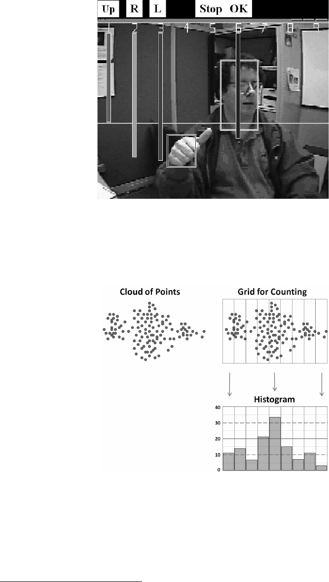
Figure 7-1: Local histograms of gradient orientations are used to find the hand and its gesture; here the

“winning” gesture (longest vertical bar) is a correct recognition of “L” (move left)

Histograms that represent continuous distributions do so by quantizing the points into each grid cell.

1

This

is where problems can arise, as shown in Figure 7-3. If the grid is too wide (upper-left), then the output is

too coarse and we lose the structure of the distribution. If the grid is too narrow (upper-right), then there is

not enough averaging to represent the distribution accurately and we get small, “spiky” cells.

Figure 7-2: Typical histogram example: starting with a cloud of points (upper-left), a counting grid is

imposed (upper-right) that yields a one-dimensional histogram of point counts (lower-right)

OpenCV has a data type for representing histograms. The histogram data structure is capable of

representing histograms in one or many dimensions, and it contains all the data necessary to track bins of

both uniform and non-uniform sizes. And, as you might expect, it comes equipped with a variety of useful

functions that allow us to easily perform common operations on our histograms.

1

This is also true of histograms representing information that falls naturally into discrete groups when the histogram

uses fewer bins than the natural description would suggest or require. An example of this is representing 8-bit intensity

values in a 10-bin histogram: each bin would then combine the points associated with approximately 25 different

intensities, (erroneously) treating them all as equivalent.