There are two
different
approaches to generating image data. The easiest way is to treat the
image as a drawing surface and use the methods of
Graphics2D to render things into the image. The
second way is to twiddle the bits of the image data yourself. This is
harder, but it can be useful in specific cases: loading and saving
images in files or mathematically analyzing image data are two
examples.
Let’s begin with the simpler approach, rendering on an image. We’ll throw in a twist, to make things interesting: we’ll build an animation. Each frame will be rendered as we go along. This is very similar to the double buffering we examined in the last chapter, but this time we’ll use a timer, instead of mouse events, as the signal to generate new frames.
Swing performs double buffering automatically, so we don’t even have to worry about the animation flickering. Although it looks like we’re drawing directly to the screen, we’re really drawing into an image that Swing uses for double buffering. All we need to do is draw the right thing at the right time.
Let’s look at an example,
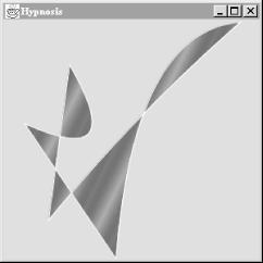
Hypnosis, that illustrates the technique. This
example shows a constantly shifting shape that bounces around the
inside of a component. When screen savers first came of
age, this kind of thing was pretty hot stuff.
Hypnosis is shown in Figure 18.2; here is its source code:
//file: Hypnosis.java
import java.awt.*;
import java.awt.event.*;
import java.awt.geom.GeneralPath;
import javax.swing.*;

public class Hypnosis extends JComponent implements Runnable {
  private int[] coordinates;
  private int[] deltas;
  private Paint paint;

  public Hypnosis(int numberOfSegments) {
    int numberOfCoordinates = numberOfSegments * 4 + 2;
    coordinates = new int[numberOfCoordinates];
    deltas = new int[numberOfCoordinates];
    for (int i = 0 ; i < numberOfCoordinates; i++) {
      coordinates[i] = (int)(Math.random( ) * 300);
      deltas[i] = (int)(Math.random( ) * 4 + 3);
      if (deltas[i] > 4) deltas[i] = -(deltas[i] - 3);
    }
    paint = new GradientPaint(0, 0, Color.blue,
        20, 10, Color.red, true);

    Thread t = new Thread(this);
    t.start( );
  }

  public void run( ) {
    try {
      while (true) {
        timeStep( );
        repaint( );
        Thread.sleep(1000 / 24);
      }
    }
    catch (InterruptedException ie) {}
  }

  public void paint(Graphics g) {
    Graphics2D g2 = (Graphics2D)g;
    g2.setRenderingHint(RenderingHints.KEY_ANTIALIASING,
        RenderingHints.VALUE_ANTIALIAS_ON);
    Shape s = createShape( );
    g2.setPaint(paint);
    g2.fill(s);
    g2.setPaint(Color.white);
    g2.draw(s);
  }

  private void timeStep( ) {
    Dimension d = getSize( );
    if (d.width == 0 || d.height == 0) return;
    for (int i = 0; i < coordinates.length; i++) {
      coordinates[i] += deltas[i];
      int limit = (i % 2 == 0) ? d.width : d.height;
      if (coordinates[i] < 0) {
        coordinates[i] = 0;
        deltas[i] = -deltas[i];
      }
      else if (coordinates[i] > limit) {
        coordinates[i] = limit - 1;
        deltas[i] = -deltas[i];
      }
    }
  }

  private Shape createShape( ) {
    GeneralPath path = new GeneralPath( );
    path.moveTo(coordinates[0], coordinates[1]);
    for (int i = 2; i < coordinates.length; i += 4)
      path.quadTo(coordinates[i], coordinates[i + 1],
          coordinates[i + 2], coordinates[i + 3]);
    path.closePath( );
    return path;
  }

  public static void main(String[] args) {
    JFrame f = new JFrame("Hypnosis");
    f.addWindowListener(new WindowAdapter( ) {
      public void windowClosing(WindowEvent we) { System.exit(0); }
    });
    Container c = f.getContentPane( );
    c.setLayout(new BorderLayout( ));
    c.add(new Hypnosis(4));
    f.setSize(300, 300);
    f.setLocation(100, 100);
    f.setVisible(true);
  }
}
The main( ) method does the usual grunt work of
setting up a JFrame
that will hold our animation component.
The Hypnosis component has a very basic strategy
for animation. It holds some number of
coordinate pairs in its
coordinates member variable. A corresponding array,
deltas, holds “delta” amounts that are
added to the coordinates each time the figure is supposed to change.
To render the complex shape you see in Figure 18.2, Hypnosis creates the
shape from the coordinates array each time the component is drawn.
Hypnosis’s constructor has two important
tasks. First, it fills up the coordinates and deltas arrays with
random values. The number of array elements is determined by an
argument to the constructor. The constructor’s second task is
to start up a new thread that will drive the animation.
The animation is
done in the run( )
method. This method calls
timeStep( )
,
which repaints the component and waits for a short time (details to
follow). Each time timeStep( ) is called, the
coordinates array is updated. Then repaint( ) is
called. This results in a call to paint( ), which
creates a shape from the coordinate array and draws it.
The paint( ) method is relatively simple. It uses
a helper method, called createShape( )
, to create a
shape from the coordinate array. The shape is then filled, using a
Paint stored as a member variable. The
shape’s outline is also drawn in white.
The timeStep( ) method updates all the elements of
the coordinate array by adding the corresponding element of deltas.
If any coordinates are now out of the components bounds, they are
adjusted and the corresponding delta is negated. This produces the
effect of bouncing off the sides of the component.
createShape( ) creates a shape from the coordinate
array. It uses the
GeneralPath
class, a useful
Shape implementation that allows you to build
shapes using straight and curved line segments. In this case, we
create a shape from a series of quadratic
curves.
So far, we’ve talked about java.awt.Images
and how they can be loaded and drawn. What if you really want to get
inside the image to examine and update its data?
Image doesn’t give you access to its data.
You’ll need to use a more sophisticated class,
java.awt.image.BufferedImage
. These classes are closely
related—BufferedImage, in fact, is a
subclass of
Image
. But BufferedImage
gives you all sorts of control over the actual data that makes up the
image. You can think of BufferedImage as an
Image on steroids. Because it’s a subclass
of Image, you can pass a
BufferedImage to any of Graphics2D’s methods
that accept an Image.
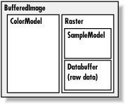
To create an image from raw data arrays, you need to understand
exactly how a BufferedImage is put together. It’s
actually quite complex—the BufferedImage
class was designed to support images in nearly any storage format you
could imagine. Figure 18.3 shows the elements
of a BufferedImage.
An image is simply a rectangle of colored
pixels, which is a simple enough
concept. There’s a lot of complexity underneath the
BufferedImage class, because there are a lot of
different ways to represent the colors of pixels. You might have, for
instance, an image with RGB data where each pixel’s red, green,
and blue values were stored as the elements of byte arrays. Or you
might have an
RGB image where each pixel was represented by
an integer that contained red, green, and blue values. Or you could
have a 16-level grayscale image with 8 pixels stored in
each element of an integer array. You get the idea—there are
many different ways to store image data, and
BufferedImage is designed to support all of them.
A BufferedImage
consists of two pieces, a
Raster and a ColorModel. The
Raster contains the actual image data. You can
think of it as an array of
pixel values. It can answer questions
like “What are the data values for the pixel at 51, 17?”
The Raster for an RGB image would return three
values, while a Raster for a grayscale image would
return a single value. A subclass of Raster,
WritableRaster, also supports modifying pixel data
values.
The ColorModel’s job is to interpret the
image data as colors. The ColorModel can translate
the data values that come from the Raster into
Color objects. An RGB color model, for example,
would know how to interpret three data values as red, green, and
blue. A grayscale color model could interpret a single data value as
a gray level. Conceptually, at least, this is how an image is
displayed on the screen. The graphics system retrieves the data for
each pixel of the image from the Raster. Then the
ColorModel tells what color each pixel should be
and the graphics system is able to set the color of each pixel.
The Raster itself is made up of two pieces, a
DataBuffer
and a SampleModel. A
DataBuffer is a wrapper for the raw data arrays,
which are byte, short, or
int arrays. DataBuffer has
handy subclasses,
DataBufferByte
, DataBufferShort, and
DataBufferInt, that allow you to create a
DataBuffer from raw data arrays. You’ll see
an example of this technique later, in the
StaticGenerator example.
The SampleModel knows how to extract the data
values for a particular pixel from the DataBuffer.
It knows the layout of the arrays in the
DataBuffer and can answer the question “What
are the data values for pixel x, y?”
SampleModels are a little tricky to work with, but
fortunately you’ll probably never need to create or use one
directly. As we’ll see, the Raster class has
many static (“factory”) methods that create preconfigured
Rasters for you, including their
DataBuffers and SampleModels.
As Figure 18.1 shows, the
2D API comes
with various flavors of ColorModels,
SampleModels, and DataBuffers.
These serve as handy building blocks that cover most common image
storage formats. You’ll rarely need to subclass any of these
classes to create a BufferedImage.
Everybody wants to work with color in their application, but using color raises problems. The most important problem is simply how to represent a color. There are many different ways to encode color information: red, green, blue (RGB) values; hue, saturation, value (HSV); hue, lightness, saturation (HLS); and more. In addition, you can provide full-color information for each pixel, or you can just specify an index into a color table (palette) for each pixel. The way you represent a color is called a color model. The 2D API provides tools to support any color model you could imagine. Here, we’ll just cover two broad groups of color models: direct and indexed.
As you might expect, you must specify a color model in order to
generate pixel data; the abstract class
java.awt.image.ColorModel represents a color
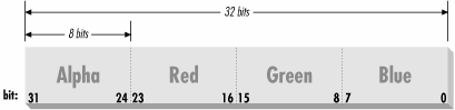
model. By default, Java 2D uses a direct color model called
ARGB. The A stands for
“alpha,” which is the historical name for transparency.
RGB refers to the red, green, and blue color components that are
combined to produce a single, composite color. In the default ARGB
model, each pixel is represented by a 32-bit integer that is
interpreted as four 8-bit fields; in order, the fields represent the
transparency (A), red, green, and blue components of the color, as
shown in Figure 18.4.
To create an instance of the
default ARGB model, call the static
getRGB-default( ) method in
ColorModel. This method returns a
DirectColorModel object;
DirectColorModel
is a subclass of
ColorModel. You can also create other direct color
models by calling a DirectColorModel constructor,
but you shouldn’t need to unless you have a fairly exotic
application.
In an indexed color model, each pixel is represented by a smaller piece of information: an index into a table of real color values. For some applications, generating data with an indexed model may be more convenient. If you have an 8-bit display or smaller, using an indexed model may be more efficient, since your hardware is internally using an indexed color model of some form.
Let’s take a look at producing some image data.
A picture may be worth a thousand words, but fortunately, we can
generate a picture in significantly fewer than a thousand words of
Java. If we just want to render image frames byte by byte, you can
put together a
BufferedImage
pretty easily.
The following application, ColorPan, creates an
image from an array of integers holding RGB pixel values:
//file: ColorPan.java
import java.awt.*;
import java.awt.event.*;
import java.awt.image.*;
import javax.swing.*;

public class ColorPan extends JComponent {
  BufferedImage image;

  public void initialize( ) {
    int width = getSize( ).width;
    int height = getSize( ).height;
    int[] data = new int [width * height];
    int i = 0;
    for (int y = 0; y < height; y++) {
      int red = (y * 255) / (height - 1);
      for (int x = 0; x < width; x++) {
        int green = (x * 255) / (width - 1);
        int blue = 128;
        data[i++] = (red << 16) | (green << 8 ) | blue;
      }
    }

    image = new BufferedImage(width, height,
        BufferedImage.TYPE_INT_RGB);
    image.setRGB(0, 0, width, height, data, 0, width);
  }

  public void paint(Graphics g) {
    if (image == null) initialize( );
    g.drawImage(image, 0, 0, this);
  }

  public static void main(String[] args) {
    JFrame f = new JFrame("ColorPan");
    f.getContentPane().add(new ColorPan( ));
    f.setSize(300, 300);
    f.setLocation(100, 100);
    f.addWindowListener(new WindowAdapter( ) {
      public void windowClosing(WindowEvent e) {
        System.exit(0);
      }
    });
    f.setVisible(true);
  }
}
Give it a try. The size of the image is determined by the size of the application window when it starts up. You should get a very colorful box that pans from deep blue at the upper-left corner to bright yellow at the bottom right, with green and red at the other extremes.
We create a BufferedImage in the
initialize( )
method and then display the image in paint( ). The
variable data is a one-dimensional array of
integers that holds 32-bit RGB pixel values. In initialize( ) we loop over every
pixel in the image and assign it an RGB
value. The blue component is always 128, half its maximum intensity.
The red component varies from 0 to 255 along the y-axis; likewise, the green component varies from 0 to 255 along the x-axis. This statement combines these components into an RGB value:
data[i++] = (red << 16) | (green << 8 ) | blue;
The
bitwise left-shift operator (<<) should be
familiar to C programmers. It simply shoves the bits over by the
specified number of positions.
When we create the BufferedImage, all its data is
zeroed out. All we specify in the constructor is the width and height
of the image and its type. BufferedImage includes
quite a few constants representing image storage types. We’ve
chosen TYPE_INT_RGB here, which indicates we want
to store the image as RGB data packed into integers. The
constructor takes care of creating an
appropriate ColorModel, Raster,
SampleModel, and DataBuffer for
us. Then we simply use a convenient method, setRGB( )
, to
assign our data to the image. In this way, we’ve side-stepped
the messy innards of BufferedImage. In the next
example, we’ll take a closer look at the details.
Once we have the image, we can draw it on the display with the familiar
drawImage( ) method.
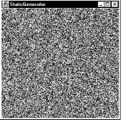
BufferedImage can also be used to
update an image dynamically. Because
the image’s data arrays are directly accessible, you can change
the data and redraw the picture whenever you want. This is probably
the easiest way to build your own low-level animation software. The
following example simulates the static on a television screen. It
generates successive
frames of random black and
white pixels and displays each frame when it is complete. Figure 18.5 shows one frame of random static; the
code follows:
//file: StaticGenerator.java
import java.awt.*;
import java.awt.event.*;
import java.awt.image.*;
import java.util.Random;
import javax.swing.*;

public class StaticGenerator extends JComponent implements Runnable {
  byte[] data;
  BufferedImage image;
  Random random;

  public void initialize( ) {
    int w = getSize().width, h = getSize( ).height;
    int length = ((w + 7) * h) / 8;
    data = new byte[length];
    DataBuffer db = new DataBufferByte(data, length);
    WritableRaster wr = Raster.createPackedRaster(db, w, h, 1, null);
    ColorModel cm = new IndexColorModel(1, 2,
        new byte[] { (byte)0, (byte)255 },
        new byte[] { (byte)0, (byte)255 },
        new byte[] { (byte)0, (byte)255 });
    image = new BufferedImage(cm, wr, false, null);
    random = new Random( );
    new Thread(this).start( );
  }

  public void run( ) {
    while (true) {
      random.nextBytes(data);
      repaint( );
      try { Thread.sleep(1000 / 24); }
      catch( InterruptedException e ) { /* die */ }
    }
  }

  public void paint(Graphics g) {
    if (image == null) initialize( );
    g.drawImage(image, 0, 0, this);
  }

  public static void main(String[] args) {
    JFrame f = new JFrame("StaticGenerator");
    f.getContentPane().add(new StaticGenerator( ));
    f.setSize(300, 300);
    f.setLocation(100, 100);
    f.addWindowListener(new WindowAdapter( ) {
      public void windowClosing(WindowEvent e) {
        System.exit(0);
      }
    });
    f.setVisible(true);
  }
}
The initialize( ) method sets up the
BufferedImage that produces the sequence of
images. We build this image from the bottom up, starting with the raw
data array. Since we’re only displaying two colors here, black
and white, we need only one bit per pixel. We want a 0 bit to represent black and a 1 bit to represent white. This calls for
an indexed color model, which we’ll create a little later.
The image data is stored as a byte array, where each array element holds eight pixels. The array length, then, is calculated by multiplying the width and height of the image and dividing by eight. We also have to adjust for the fact that each image row starts on a byte boundary. For example, an image that was 13 pixels wide would actually use 2 bytes (16 bits) for each row:
int length = ((w + 7) * h) / 8;
Next, the actual byte array is created. The member variable data
holds a reference to this array. Later, we’ll use data to
change the image data dynamically. Once we have the image data array,
it’s easy to create a
DataBuffer
from it:
data = new byte[length];
DataBuffer db = new DataBufferByte(data, length);
DataBuffer has several subclasses, like
DataBufferByte, that make it easy to create a data
buffer from raw arrays.
The next step, logically, is to create a
SampleModel
. Then we could create a
Raster from the SampleModel and
the DataBuffer. Lucky for us, though, the
Raster
class contains a bevy of useful
static methods that create common types of
Rasters. One of these methods creates a
Raster from data that contains multiple pixels
packed into array elements. We simply use this method, supplying the
data buffer, the width and height, and indicating that each pixel
uses one bit:
WritableRaster wr = Raster.createPackedRaster(db, w, h, 1, null);
The last argument to this method is a Point that
indicates where the upper-left corner of the
Raster should be. By passing null, we use the
default of 0, 0.
The last piece of the puzzle is the ColorModel.
Each pixel is either 0or 1, but how should that be interpreted as color? In this case, we use an IndexColorModel
with a very small palette. The palette has only two entries, one each for black and white:
ColorModel cm = new IndexColorModel(1, 2,
        new byte[] { (byte)0, (byte)255 },
        new byte[] { (byte)0, (byte)255 },
        new byte[] { (byte)0, (byte)255 });
The IndexColorModel constructor that we’ve
used here accepts the number of bits per pixel (1), the number of
entries in the palette(2), and three byte arrays that are the red,
green, and blue components of the palette colors. Our palette
consists of two colors: black (0, 0, 0) and white (255, 255, 255).
Now that we’ve got all the pieces, we just need to create a
BufferedImage. This image is also stored in a
member variable so we can draw it later. To create the
BufferedImage, we pass the color model and
writable raster we just created:
image = new BufferedImage(cm, wr, false, null);
All the hard work is done now. Our paint( ) method
just draws the image, using drawImage( ).
The init( ) method starts a thread that generates
the pixel data. The run( ) method takes care of
generating the pixel data. It uses a Random object to fill the data
image data array with random values. Since the data array is the
actual image data for our image, changing the data values changes the
appearance of the image. Once we fill the array with random data, a
call to repaint( ) shows the new image on the
screen.
That’s about all there is. It’s worth noting how simple
it is to create this animation. Once we have the
BufferedImage, we treat it like any other image.
The code that generates the image sequence can be arbitrarily
complex. But that complexity never infects the
simple task of
getting the image
on the screen and updating it.
Get Learning Java now with the O’Reilly learning platform.
O’Reilly members experience books, live events, courses curated by job role, and more from O’Reilly and nearly 200 top publishers.

