Chapter 4. Querying Delimited Data
In this chapter we get started with Apache Drill by querying simple data. We are defining “simple data” as data contained in a delimited file such as a spreadsheet or comma-separated values (CSV) file, from a single source. If you have worked with SQL databases, you will find that querying simple data with Drill is not much different than querying data from a relational database. However, there are some differences that are important to understand in order to unleash the full power of Drill. We assume that you are familiar with basic SQL syntax, but if you are not, we recommend SQL Queries for Mere Mortals (Addison-Wesley) by John Viescas as a good SQL primer.
To follow along, start Drill in embedded mode as explained in Chapter 2 and download the example files, which are available in the GitHub repository for this book.
Ways of Querying Data with Drill
Drill is very flexible and provides you with several different ways of querying data. You’ve already seen that Drill has a command-line interface known as SQLLine. In addition to the command line, Drill has a web interface that you can access by opening a browser (after Drill is running) and navigating to http://localhost:8047, as shown in Figure 4-1.
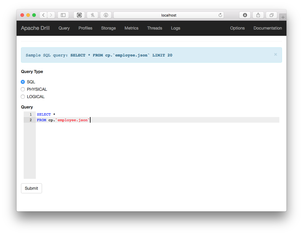
Figure 4-1. The Drill Web Console
Other Interfaces
You can also query data with Drill by using Drill’s RESTful interface or by using a conventional tool such as Tableau and using Drill’s ODBC or JDBC interfaces. We cover these interfaces later in the book and demonstrate how to query Drill using your favorite scripting languages, such as Python or R.
Lastly, if you install the MapR ODBC driver for Drill, bundled with that is a tool called Drill Explorer, which is another GUI for querying Drill.
For the beginning examples, we recommend that you start out by using the Web Console because there are certain features that are most easily accessed through it.
Drill SQL Query Format
Drill uses the ANSI SQL standard with some extensions around database table and schema naming. So, if you are comfortable with relational databases most of Drill’s SQL syntax will look very familiar to you. Let’s begin with a basic query. Every SQL SELECT query essentially follows this format:
SELECTlist_of_fieldsFROMone_or_more_tablesWHEREsome_logical_conditionGROUPBYsome_field
As in standard SQL, the SELECT and FROM clauses are required, the WHERE and GROUP BY clauses are optional. Again, this should look relatively familiar to you, and this chapter will focus on Drill’s unique features in SQL.
Choosing a Data Source
In most ways, Drill behaves like a traditional relational database, with the major difference being that Drill treats files (or directories) as tables. Drill can also connect to relational databases or other structured data stores, such as Hive or HBase, and join them with other data sources, but for now, let’s look at querying a simple CSV file in Drill:
SELECTfirst_name,last_name,street_address,ageFROMdfs.user_data.`users.csv`WHEREage>21
This queries a sample data file called users.csv and returns the first name, last name, and street address of every user whose age is greater than 21. If you are familiar with relational databases, the only part that might look unusual is this line:
FROMdfs.user_data.`users.csv`
In a traditional database, the FROM clause contains the names of tables, or optionally the names of additional databases and associated tables. However, Drill treats files as tables, so in this example, you can see how to instruct Drill which file to query.
Drill accesses data sources using storage plug-ins, and the kind of system your data is stored in will dictate which storage plug-in you use. In Drill, the FROM clause has three components that do slightly different things depending on what kind of storage plug-in you are using. The components are the storage plug-in name, the workspace name, and the table name. In the previous example, dfs is one of the default storage plug-ins; “dfs” stands for distributed filesystem and is used to access data from sources such as HDFS, cloud storage, and files stored on the local system.1 The next component is optional; it’s the workspace, which is a shortcut to a file path on your system. If you didn’t want to use a workspace, you could enter the following:
FROMdfs.`full_file_path/users.csv`
Finally, there is the table, which this storage plug-in corresponds to a file or directory. In addition to the dfs plug-in, Drill ships with the cp or classpath plug-in enabled, which queries files stored in one of the directories in your Java classpath, typically used to access the example files included with Drill.
As illustrated in Figure 4-2, the Storage Configuration panel is where you can enable, disable, and configure the various storage plug-ins. You should resist the temptation to enable all the disabled plug-ins because you will get bad performance and strange error messages if you try to use Drill with an improperly configured storage plug-in enabled.
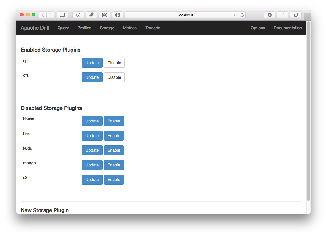
Figure 4-2. Drill storage plug-in configuration
Defining a Workspace
In Drill parlance, when you are using file-based systems, a workspace is a shortcut to a file path. To create a workspace, open the Drill web interface and then, at the top of the screen, click the Storage tab.
Next, click the Update button next to the dfs plug-in (see Figure 4-2) and you will see the configuration variables. You will see a section called workspaces, and there you will see the default workspaces, root and tmp, as shown here:
"workspaces":{"root":{"location":"/","writable":false,"defaultInputFormat":null},"tmp":{"location":"/tmp","writable":true,"defaultInputFormat":null}},
To create your own workspace, simply add another entry into the workspaces section with a path to a location on your local filesystem:
"drill_tutorial":{"location":"your_path","writable":true,"defaultInputFormat":null}
You must have read permission to be able to read data in your workspace, and it goes without saying that if you want to write to this path, you must have write permissions. You can configure workspaces as being writable or not, as well as setting a default file format. Often you will want to take the results of complex queries and create tables or views, and the workspace must be writable in order to store a view or new table. After you’ve created your workspace, at the bottom of the screen, click the Update button.
You can verify that your workspace was successfully created by executing a SHOW DATABASES statement; you should see your newly created workspace in the results.
View Your Configuration by Using the DESCRIBE Statement
In addition to the SHOW DATABASES statement, you can also view the plug-in configuration by using the DESCRIBE SCHEMA statement. For instance, you can view the configuration used in a notional workspace called test by using the statement DESCRIBE SCHEMA dfs.test.
Specifying a Default Data Source
The examples thus far use file paths in the FROM clause. In practice, these clauses can become long, and it is tedious to type them over and over in an interactive session. Drill has the idea of a default data source, which is used if you don’t specify a data source (storage plug-in and workspace, also called a namespace) in your query. You use the USE statement to select the data source to use as the default, as shown here for dfs.data:
USEdfs.data;SELECT*FROM`users.csv`WHEREage>20
So, the preceding query is functionally equivalent to the query that follows.
SELECT*FROMdfs.data.`users.csv`WHEREage>20
SQL Sessions
Drill is a SQL tool. SQL uses the idea of a session that is tied to a Drill connection. Session state, such as the USE statement, applies only to that one session.
JDBC, ODBC, and most BI tools create sessions; however, Drill’s Web Console does not, and therefore the USE operator will not work in the Web Console. The Web Console uses Drill’s RESTful interface. When you execute queries using the RESTful interface, each query is executed in its own session and the USE statement unhelpfully lasts only for the single REST request in which it was submitted.
Saving Your Settings
By default, in embedded mode Drill saves all settings in the /tmp directory, which often does not persist if the machine is rebooted. To save your settings while running in embedded mode, you will need to modify the drill-override.conf file, which is located in the DRILL_HOME/conf/ folder, by adding the following:
sys.store.provider.local.path="path to directory"
to the section drill.exec and supplying a nontemporary path, as shown here:
drill.exec:{cluster-id:"drillbits1",zk.connect:"localhost:2181",sys.store.provider.local.path="path_to_save_file"}
It is a better practice to set up a single-node Drill cluster with ZooKeeper to save state correctly. When running Drill in server mode, Drill saves state in ZooKeeper so that it can be shared by multiple Drillbits and can be persisted across server restarts.
After you have specified a namespace with the USE operator, you can still access other namespaces, but you will need to explicitly list them, as shown here:
USEdfs.dataSELECT*FROM`users.csv`ASuINNERJOINdfs.logs.`logfile.txt`ASlONl.id=u.id
You can see in this example that the query joins data from users.csv with another file called logfile.txt, which is in a completely different namespace.
Accessing Columns in a Query
Relational databases are considered schema-on-write in that the schema must be defined prior to writing the data on disk. More recently, tools such as Apache Spark use a technique called schema-on-read, which allows more flexibility because it allows users to modify the schema as the data is being ingested rather than being tied to a rigid, predefined schema.
Drill takes a different approach and relies on the data’s natural structure for its queries. Suppose that we have a file called customer_data.csv that contains three columns of data: first_name, last_name, and birthday. Drill infers the schema directly from the structure of the data and, as such, you do not need to define any kind of schema prior to querying your data with Drill.
As an example, Drill will allow you to query this data directly by simply executing the following query:
SELECT*FROMdfs.drill_tutorial.`customer_data.csv`
However, when you execute this query you will notice that Drill returns a single column for each row of data. This one column is called columns and is an array of VARCHAR as shown in the following table:
| columns |
|---|
["Robert","Hernandez","5/3/67"] |
["Steve","Smith","8/4/84"] |
["Anne","Raps","9/13/91"] |
["Alice","Muller","4/15/75"] |
Drill infers a schema directly from your data. In this case, we have a CSV file without column headings. Since Drill doesn’t know the name or number of fields, it instead returns the fields as an array. (We will see shortly how column headings change the results.) This represents a major difference between Drill and relational databases: Drill supports nested data structures such as arrays and maps, whereas conventional relational databases do not. In Drill, just as in many other programming languages, arrays are zero-indexed, meaning that the first item in an array is the 0th item. Individual array items are accessed by using notation similar to most programming languages:
arrayName[n]
Where n is the numeric index of the item that you want to access. Although CSV uses a single array, other data sources (such as JSON) can contain a mix of nested columns and flat columns.
Getting back to our delimited data file, if you want to access the individual columns within this array, you will need to use the columns array in your query. Prior to Drill 1.15, the name columns must be in lowercase. The query that follows demonstrates how to access these columns within a query and filter data using one of these fields:
SELECTcolumns[0]ASfirst_name,columns[1]ASlast_name,columns[2]ASbirthdayFROMdfs.drill_tutorial.`customer_data.csv`WHEREcolumns[1]='Smith'
This example first creates simple columns for some of the fields by using the AS clause. In SQL terminology, doing so projects the array elements to new columns. This query would return the data shown in the following table:
| first_name | last_name | birthday |
|---|---|---|
Robert |
Hernandez |
5/3/67 |
Steve |
Smith |
8/4/84 |
Anne |
Raps |
9/13/91 |
Alice |
Muller |
4/15/75 |
Delimited Data with Column Headers
If your delimited file contains headers with the column names in the first row, you can configure Drill to read those names, as well. To do this, you will need to open the web interface and go back to the screen where you configured the storage plug-in. In this case, click the button to edit the dfs plug-in and then scroll down until you see the section labeled formats. You should see some JSON that looks like this:
"formats":{"psv":{"type":"text","extensions":["tbl"],"delimiter":"|"},"csv":{"type":"text","extensions":["csv"],"delimiter":","},...,"csvh":{"type":"text","extensions":["csvh"],"extractHeader":true,"delimiter":","}
Drill includes a number of format plug-ins that parse data files and map data to Drill fields. The "text" format is the generic delimited data plug-in and provides you with a number of options to configure how Drill will read your files. Drill lets you give names to different collections of options, such as the "psv", "csv", and other formats in the previous example (see Table 4-2).
| Options | Description |
|---|---|
comment |
Character used to start a comment line (optional) |
escape |
Character used to escape the quote character in a field |
delimiter |
Character used to delimit fields |
quote |
Character used to enclose fields |
skipFirstLine |
Skips the first line of a file if set to true (can be true or false) |
extractHeader |
Reads the header from the CSV file if set to true (can be true or false) |
If you would like Drill to extract the headers from the file, simply add the line "extractHeader": true, to the section in the configuration that contains the file type that you are working on. Drill also ships configured with the .csvh file type configured to accept CSV files with headers. To use this, simply rename your CSV files .csvh. If you want to try this out for yourself, execute this query:
SELECT*FROMdfs.drill_tutorial.`customer_data-headers.csvh`
This yields the results shown in the following table:
| first_name | last_name | birthday |
|---|---|---|
Robert |
Hernandez |
5/3/67 |
Steve |
Smith |
8/4/84 |
Anne |
Raps |
9/13/91 |
Alice |
Muller |
4/15/75 |
Table Functions
You should use the configuration options listed in Table 4-2 to set the configuration for a given storage plug-in or directory. However, you can also change these options in a query for a specific file, by using a Drill table function as seen here:
SELECT*FROMtable(dfs.drill_tutorial.`orders.csv`(type=>'text',extractHeader=>true,fieldDelimiter=>','))
When you use a table function, the query does not inherit any default values defined in the storage plug-in configuration, and thus you need to specify values for all the mandatory options for the format. In the previous example, the fieldDelimiter field is required.
Querying Directories
In addition to querying single files, you also can use Drill to query directories. All of the files in the directory must have the same structure, and Drill effectively performs a union on the files. This strategy of placing data into nested folders is known as partitioning and is very commonly used in big data systems in lieu of indexes.
Querying a directory is fundamentally no different than querying a single file, but instead of pointing Drill to an individual file, you point it to a directory. Suppose that you have a directory called logs that contains subdirectories for each year, which finally contain the actual log files. You could query the entire collection by using the following query:
SELECT*FROMdfs.`/var/logs`
If your directory contains subdirectories, you can access the subdirectory names by putting the dirN into the query. Thus, dir0 would be the first-level directory, dir1 the second, and so on. For instance, suppose that you have log files stored in directories nested in the following format:
logs
|__ year
    |__month
       |__day
You could access the directory structure by using the following query:
SELECTdir0AS`year`,dir1AS`month`,dir2AS`day`FROMdfs.`/var/logs/`
Additionally, you can use wildcards in the directory name. For instance, the following query uses wildcards to restrict Drill to opening only CSV files:
SELECT*FROMdfs.`/user/data/*.csv`
Data Partitioning Depends on the Use Cases
The directory structure in this example is from an actual example from a client; however, this is not a good way to structure partitions to work with Drill because it makes querying date ranges very difficult as we discuss in Chapter 8. One better option might be to partition the data by date in ISO format. Ultimately, it depends on what you are trying to do with your data.
Directory functions
If you are using the dir variables with the MAX() or MIN() functions in the WHERE clause in a SQL query, it is best to use the directory functions rather than simple comparisons because it allows Drill to avoid having to make costly (and slow) full-directory scans. Drill has four directory functions:
-
MAXDIR() -
MINDIR() -
IMAXDIR() -
IMINDIR()
These functions return the minimum or maximum values in a directory; IMAXDIR() and IMINDIR() return the minimum or maximum in case-insensitive order.
Directory Functions Have Limitations
The Drill directory functions perform a string comparison on the directory names. If you are trying to find the most recent directories, you cannot use these functions unless the most recent occurs first or last when compared as a string.
Using the previous example structure, the following query would find the most recent year’s directory in the logs directory and return results from that directory:
SELECT*FROMdfs.`/var/logs`WHEREdir0=MAXDIR('dfs/tmp','/var/logs')
Understanding Drill Data Types
One of the challenges in using Drill is that although it in many ways acts like a relational database, there are key areas in which it does not, and understanding these is key to getting the most out of Drill. This section will cover the fundamentals of analyzing delimited data with Drill. The examples in this section use a sample data file, baltimore_salaries_2015.csvh, which is included in the GitHub repository.2
Although Drill can infer the structure of data from the files, when you are querying delimited data Drill cannot implicitly interpret the data type of each field, and because there are no predefined schemas, you will need to explicitly cast data into a particular data type in your queries to use it for other functions. For instance, the following query fails because Drill cannot infer that the AnnualSalary field is a numeric field:
SELECTAnnualSalary,FROMdfs.drill_tutorial.`csv/baltimore_salaries_2015.csvh`WHEREAnnualSalary>35000
This query fails with a NumberFormatException because the AnnualSalary field is a string. You can check the column types by using the typeof(<column>) function as shown in the following query:
SELECTAnnualSalary,typeof(AnnualSalary)AScolumn_typeFROMdfs.drill_tutorial.`baltimore_salaries_2015.csvh`LIMIT1
This query produces the following result:
| GrossPay | column_type |
|---|---|
|
|
|
To fix this problem, you need to explicitly instruct Drill to convert the AnnualSalary field to a numeric data type. To use a comparison operator, both sides of the equation will need to be numeric, and to convert the field to a numeric data type, you will need to use the CAST(field AS data_type) function.
Table 4-3 lists the simple data types that Drill supports.
| Drill data types | Description |
|---|---|
BIGINT |
8-byte signed integer in the range –9,223,372,036,854,775,808 to 9,223,372,036,854,775,807 |
BINARY |
Variable-length byte string |
BOOLEAN |
true or false |
DATE |
Date |
DECIMAL(p,s) |
38-digit precision number; precision is p and scale is s |
DOUBLE |
8-byte floating-point number |
FLOAT |
4-byte floating-point number |
INTEGER or INT |
4-byte signed integer in the range –2,147,483,648 to 2,147,483,647 |
TIME |
Time |
TIMESTAMP |
JDBC timestamp in year, month, date hour, minute, second, and optional milliseconds |
VARCHAR |
UTF8-encoded variable-length string; the maximum character limit is 16,777,216 |
We discuss the date/time functions as well as complex data types later in the book, but it is important to understand these basic data types to do even the simplest calculations.
Suppose you would like to calculate some summary statistics about the various job roles present in this city. You might begin with a query like this:
SELECTJobTitle,AVG(AnnualSalary)ASavg_payFROMdfs.drillbook.`baltimore_salaries_2016.csvh`GROUPBYJobTitleORDERBYavg_payDESC
However, in Drill, this query will fail for the same reason as the earlier query: the GrossPay is not necessarily a number and thus must be converted into a numeric data type. The corrected query would be as follows:
SELECTJobTitle,AVG(CAST(AnnualSalaryASFLOAT))ASavg_payFROMdfs.drillbook.`baltimore_salaries_2016.csvh`GROUPBYJobTitleORDERBYavg_payDESC
However, this query will unfortunately also fail because there are extraneous characters such as the $ in the AnnualSalary field. To successfully execute this query, you can either use the TO_NUMBER() function, as explained in the next section, or use one of Drill’s string manipulation functions to remove the $. A working query would be:
SELECTJobTitle,AVG(CAST(LTRIM(AnnualSalary,'\$')ASFLOAT))ASavg_payFROMdfs.drillbook.`baltimore_salaries_2016.csvh`GROUPBYJobTitleORDERBYavg_payDESC
A cleaner option might be to break this up using a subquery, as shown here:
SELECTJobTitle,AVG(annual_salary)ASavg_payFROM(SELECTJobTitle,CAST(LTRIM(annual_salary,'\$')ASFLOAT)ASannual_salaryFROMdfs.drillbook.`baltimore_salaries_2016.csvh`)GROUPBYJobTitleORDERBYavg_payDESC
Cleaning and Preparing Data Using String Manipulation Functions
When querying data in Drill, often you will want to extract a data artifact from a source column. For instance, you might want to extract the country code from a phone number. Drill includes a series of string manipulation functions that you can use to prepare data for analysis. Table 4-4 contains a listing of all the string manipulation functions in Drill.
| Function | Return type | Description |
|---|---|---|
|
|
|
Returns in binary format a substring of a string |
|
|
|
Returns the number of characters in a string |
|
|
|
Concatenates strings |
|
|
|
Returns |
|
|
|
Returns a string with the first letter of each word capitalized |
|
|
|
Returns the length of a string |
|
|
|
Converts a string to lowercase |
|
|
|
Pads a string to the specified length by prepending the fill or a space |
|
|
|
Removes characters in string 2 from the beginning of string 1 |
|
|
|
Returns the index of the needle string in the haystack string |
|
|
|
Replaces text in the source that matches the pattern with the replacement text |
|
|
|
Pads a string to the specified length by appending the fill or a space |
|
|
|
Removes characters in string 2 from the end of string 1 |
|
|
Array of |
Splits a string on the character argument |
|
|
|
Returns the index of the needle string in the haystack string |
|
|
|
Extracts a portion of a string from a position 1– |
|
|
|
Removes characters in string 1 from string 2 |
|
|
|
Converts a string to uppercase |
A use case for some of these functions might be trying to determine which domains are most common among a series of email addresses. The available data just has the email addresses; to access the domain it will be necessary to split each one on the @ sign. Assuming that we have a field called email, the function SPLIT(email, '@') would split the column and return an array containing the accounts and domains. Therefore, if we wanted only the domains, we could add SPLIT(email, '@')[1] to the end, which would perform the split and return only the last half. Thus, the following query will return the domain and the number of users using that domain:
SELECTSPLIT(,'@')[1]ASdomain,COUNT(*)ASuser_countFROMdfs.book.`contacts.csvh`GROUPBYSPLIT(,'@')[1]ORDERBYuser_countDESC
Complex Data Conversion Functions
If you have data that is relatively clean, the CAST() function works well; however, let’s look at a real-life situation in which it will fail and how to correct that problem with the TO_ methods.
Let’s look again at the baltimore_salaries_2015.csvh file. This data contains two columns with salary data: AnnualSalary and GrossPay. However, if you wanted to do any kind of filtering or analysis using these columns, you’ll notice that we have two problems that will prevent you from performing any kind of numeric operation on them:
-
Each salary begins with a dollar sign ($).
-
Each salary also has a comma separating the thousands field.
You already used string manipulation functions and CAST() to clean the data. This time, you will use the TO_NUMBER(field, format) function, which accomplishes both tasks in one step.
Table 4-5 lists the special characters that the format string accepts.
| Symbol | Location | Meaning |
|---|---|---|
|
|
Number |
Digit. |
|
|
Number |
Digit, zero shows as absent. |
|
|
Number |
Decimal separator or monetary decimal separator. |
|
|
Number |
Minus sign. |
|
|
Number |
Grouping separator. |
|
|
Number |
Separates mantissa and exponent in scientific notation. Does not need to be quoted in prefix or suffix. |
|
|
Subpattern boundary |
Separates positive and negative subpatterns. |
|
|
Prefix or suffix |
Multiplies by 100 and shows as percentage. |
|
|
Prefix or suffix |
Multiplies by 1,000 and shows as per-mille value. |
|
|
Prefix or suffix |
Currency sign, replaced by currency symbol. If doubled, replaced by international currency symbol. If present in a pattern, the monetary decimal separator is used instead of the decimal separator. |
|
|
Prefix or suffix |
Used to quote special characters in a prefix or suffix; for example, |
Therefore, to access the salary columns in the Baltimore Salaries data, you could use the following query:
SELECTTO_NUMBER(AnnualSalary,'¤000,000')ASActualPayFROMdfs.drill_tutorial.`baltimore_salaries_2015.csvh`WHERETO_NUMBER(AnnualSalary,'¤000,000')>=50000
Working with Dates and Times in Drill
Similar to numeric fields, if you have data that has dates or times that you would like to analyze, you first need to explicitly convert them into a format that Drill recognizes. For this section, we use a file called dates.csvh, which contains five columns of random dates in various formats (see Figure 4-3).

Figure 4-3. Results of a date/time query
There are several ways of converting dates into a usable format, but perhaps the most reliable way is to use the TO_DATE(expression, format) function. This function takes two arguments: an expression that usually will be a column, and a date format that specifies the formatting of the date that you are reading. Unlike many relational databases, Drill typically uses Joda—aka Java 8 Date Time or java.time format—formatting for the date strings for all date/time functions; however, there are several functions to convert dates that support ANSI format.3 See Appendix A for a complete list of Drill functions, and see Table B-2 for a list of Joda date/time formatting characters.
Converting Strings to Dates
To demonstrate how to convert some dates, in the file dates.csvh you will see that there are five columns with random dates in the following formats:
date1-
ISO 8601 format
date2-
Standard “American” date with month/day/year
date3-
Written date format: three-letter month, date, year
date4-
Full ISO format with time zone and day of week
- date5
-
MySQL database format (yyyy-mm-dd)
The first one is easy. Drill’s native CAST() function can interpret ISO 8601–formatted dates, so the following query would work:
SELECTCAST(date1ASDATE)FROMdfs.drill_tutorial.`dates.csvh`
The second column is a little trickier. Here, the month is first and the day is second. To ingest dates in this format, you need to use the TO_DATE(expression, format_string) function, as shown here:
SELECTdate2,TO_DATE(date2,'MM/dd/yyyy')FROMdfs.drill_tutorial.`dates.csvh`
The third column contains dates that are formatted more in “plain text”: Sep 18, 2016, for instance. For these dates you also need to use the TO_DATE() function, but with a slightly different format string:
SELECTdate3,TO_DATE(date3,'MMM dd, yyyy')FROMdfs.drill_tutorial.`dates.csvh`
The fourth column introduces some additional complexity in that it has a time value as well as a time zone, as you can see here: Sun, 19 Mar 2017 00:15:28 –0700. It can be ingested using the TO_DATE() function; however, in doing so, you will lose the time portion of the timestamps. Drill has a function called TO_TIMESTAMP() that is similar to TO_DATE() but retains the time components of a date/time:
SELECTdate4,TO_TIMESTAMP(date4,'EEE, dd MMM yyyy HH:mm:ss Z')FROMdfs.drill_tutorial.`dates.csvh`
The final column in this exercise, date5, has dates in the format of yyyy-MM-dd, which is very commonly found in databases. You can parse it easily using the TO_DATE() function, as shown in the following query:
SELECTdate5,TO_DATE(date5,'yyyy-MM-dd')FROMdfs.drill_tutorial.`dates.csvh`
Reformatting Dates
If you have a date or a time that you would like to reformat for a report, you can use the TO_CHAR(date/time_expression, format_string) function to convert a Drill date/time into a formatted string. Like the TO_DATE() function, TO_CHAR() uses Joda date formatting. Table 4-6 presents the Drill date conversion functions.
| You have a... | You want a... | Use... |
|---|---|---|
|
|
DATE |
|
|
|
TIME |
|
|
DATE |
VARCHAR |
|
Date Arithmetic and Manipulation
Much like other databases, Drill has the ability to perform arithmetic operations on dates and times; however, Drill has a specific data type called an INTERVAL that is returned whenever you perform an operation on dates. When converted to a VARCHAR, an INTERVAL is represented in the ISO 8601 duration syntax as depicted here:
P [quantity] Y [quantity] M [quantity] D T [quantity] H [quantity] M [quantity] S
P [quantity] D T [quantity] H [quantity] M [quantity] S
P [quantity] Y [quantity] M
It is important to understand this format because it is returned by every function that makes some calculation on dates. To try this out, using the dates.csvh file discussed earlier, the following query calculates the difference between two date columns:
SELECTdate2,date5,(TO_DATE(date2,'MM/dd/yyyy')-TO_DATE(date5,'yyyy-MM-dd'))asdate_diffFROMdfs.drill_tutorial.`dates.csvh`
The resulting date_diff column contains values such as these:
-
P249D -
P-5D -
P-312D
You can extract the various components of the INTERVAL by using the EXTRACT() function, the syntax for which is EXTRACT(part FROM field).
Date and Time Functions in Drill
Drill has a series of date and time functions that are extremely useful in ad hoc data analysis and exploratory data analysis, which you can see listed in Table 4-7.
| Function | Return type | Description |
|---|---|---|
|
|
|
Returns the age of the given time expression. |
|
|
|
Returns the current date. |
|
|
|
Returns the current time. |
|
|
|
Returns the current timestamp. |
|
|
|
Returns the sum of the date and the second argument. This function accepts various input formats. |
|
|
|
Returns a portion of a date expression, specified by the keyword. |
|
|
|
Returns the difference between the date and the second argument. This function accepts various input formats. |
|
|
|
Extracts and returns a part of the given date expression or interval. |
|
|
|
Returns the local time. |
|
|
|
Returns the current local time. |
|
|
|
Returns the current local time. |
|
|
|
|
|
|
|
Returns a Unix timestamp of the current time if a date string is not specified, or the Unix timestamp of the specified date. |
Time Zone Limitation in Drill
At the time of writing, Drill does not support converting dates from one time zone to another. Drill uses the time zone from your operating system unless you override it, which can cause inconsistencies in your analysis if you are looking at data with timestamps from different time zones.
The best workaround at this point is to set up Drill to use UTC and to convert all your data to UTC, as well. To set Drill to use UTC you need to add the following line to the drill-env.sh file in the DRILL_PATH/conf/ folder.
export DRILL_JAVA_OPTS=\
"$DRILL_JAVA_OPTS -Duser.timezone=UTC"
After you’ve done that, restart Drill and any Drillbits that might be running and then execute the following query to verify that Drill is running in UTC time:
SELECTTIMEOFDAY()FROM(VALUES(1))
Creating Views
Like many relational databases, Drill supports the creation of views. A view is a stored query that can include many data sources, functions, and other transformations of the data. You can use views to simplify queries, control access to your data, or even mask portions of it. As with relational databases, creating a view does not store the actual data, only the SELECT statement to retrieve the data.
Here’s the basic syntax to create a view:
CREATE[ORREPLACE]VIEWworkspace.view_nameASquery
You can also specify the columns after the view name. If you do not do this, the column names will be extrapolated from the query. After you have created a view, you can use the view name in the query as if it were a regular table.
For instance, let’s say that you have a CSV file called orders.csvh, and you want to create a view of this data with data types already specified. You could use the following query to do so:
CREATEVIEWdfs.customers.order_dataASSELECTcolumns[1]customer__first_name,columns[2]AScustomer_last_name,CAST(columns[3]ASINT)ASproduct_idcolumns[4]ASproduct_nameCAST(columns[5]ASFLOAT)ASpriceFROMdfs.data.`orders.csv`
Let’s also say that you wanted to find each customer’s average purchase amount. You could find that with the following query:
SELECTcustomer_last_name,customer_first_name,AVG(price)FROMdfs.customers.order_dataGROUPBYcustomer_last_name,customer_first_name
In this example, by creating a view, you can eliminate all the data type conversions and assign readable field names to the data.4
Data Analysis Using Drill
Now that you know how to get Drill to recognize dates as well as numeric fields, you are ready to begin analyzing data. Much like any database, Drill has a variety of mathematical functions that you can use in the SELECT statements to perform calculations on your data. You can apply one of these functions to a column or nest functions, and the result will be a new column. Table 4-8 shows the operations that Drill currently supports.
| Function | Return type | Description |
|---|---|---|
|
|
Same as input |
Returns the absolute value of the input argument |
|
|
|
Returns the cubic root of |
|
|
Same as input |
Returns the smallest integer not less than |
|
|
Same as input |
Same as |
|
|
|
Converts |
|
|
|
Returns 2.718281828459045. |
|
|
|
Returns e (Euler’s number) to the power of |
|
|
Same as input |
Returns the largest integer not greater than |
|
|
|
Returns the natural log (base e) of |
|
|
|
Returns log base |
|
|
|
Returns the common log of |
|
|
Same as input |
Shifts the binary |
|
|
|
Returns the remainder of |
|
|
Same as input |
Returns |
|
|
|
Returns pi. |
|
|
|
Returns the value of |
|
|
|
Converts |
|
|
|
Returns a random number from 0–1. |
|
|
Same as input |
Rounds to the nearest integer. |
|
|
DECIMAL |
Rounds |
|
|
Same as input |
Shifts the binary |
|
|
INT |
Returns the sign of |
|
|
Same as input |
Returns the square root of |
|
|
Same as input |
Truncates |
|
|
DECIMAL |
Truncates |
All of these functions require the inputs to be some numeric data type, so don’t forget to convert your data into a numeric format before using one of these columns. The following example demonstrates how to calculate the square root of a column using Drill’s SQRT() function:
SELECTx,SQRT(CAST(xASFLOAT))ASsqrt_xFROMdfs.data.csv
Table 4-9 presents the results.
| x | sqrt_x |
|---|---|
|
4 |
2 |
|
9 |
3 |
|
16 |
4 |
Summarizing Data with Aggregate Functions
In addition to the standard mathematical functions, Drill also includes the aggregate functions that follow, which perform a calculation on an entire column or grouping within a column. These functions are extremely useful when summarizing a dataset. A complete explanation of grouping in SQL is available in Chapters 13 and 14 of Viesca’s SQL Queries for Mere Mortals (Addison-Wesley). However, the essential structure of a query that summarizes data is as follows:
SELECTuniquefield,aggregatefunction(field)FROMdataWHERElogicalcondition(Optional)GROUPBYuniquefieldorfieldsHAVINGlogicalcondition(Optional)
You can use aggregate functions to summarize a given column, and in these instances the aggregate function will return one row. Table 4-10 lists the aggregate functions included with Drill as of this writing.
| Function | Return type | Description |
|---|---|---|
|
|
Same as argument type |
Returns the average of the expression |
|
|
|
Returns the number of rows |
|
|
|
Returns the number of unique values and the number of times they occurred |
|
|
Same as argument type |
Returns the smallest value in the expression |
|
|
|
Returns the sample standard deviation of the column |
|
|
|
Returns the population standard deviation of the input column |
|
|
|
Returns the sample standard deviation of the input column |
|
|
Same as argument type |
Returns the sum of the given column |
|
|
|
Returns the sample variance of the input values (sample standard deviation squared) |
|
|
|
Returns the population variance of the input values (the population standard deviation squared) |
|
|
|
Sample variance of input values (sample standard deviation squared) |
As an example, this book’s GitHub repository contains a data file called orders.csvh which contains notional sales data for one month. If you wanted to calculate some monthly stats, you could use the following query to do so:
SELECTSUM(CAST(purchase_amountASFLOAT))ASmonthly_total,MAX(CAST(purchase_amountASFLOAT))ASlargest_order,MIN(CAST(purchase_amountASFLOAT))ASsmallest_order,COUNT(order_id)ASorder_count,AVG(CAST(purchase_amountASFLOAT))ASaverage_orderFROMdfs.drill_tutorial.`orders.csvh`
Figure 4-4 shows the results.
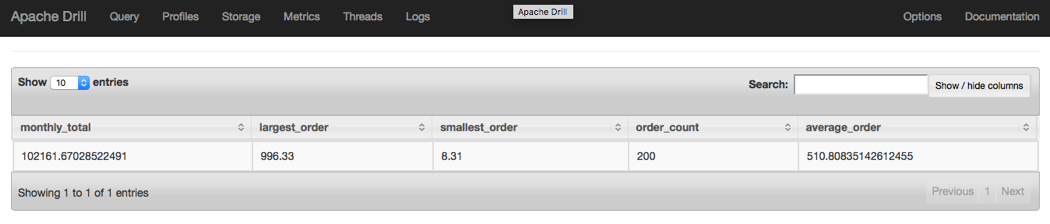
Figure 4-4. Stats query result
As you can see, the query calculates the total monthly sales, the largest order, the smallest order, the number of orders, and the average order amount for the month.
If you wanted to summarize this data by day, all you would need to do is add a GROUP BY statement at the end of the query, as shown in the following example:
SELECTEXTRACT(dayFROMTO_DATE(order_date,'yyyy-MM-dd'))ASday_of_month,SUM(CAST(purchase_amountASFLOAT))ASdaily_total,MAX(CAST(purchase_amountASFLOAT))ASlargest_order,MIN(CAST(purchase_amountASFLOAT))ASsmallest_order,COUNT(order_id)ASorder_count,AVG(CAST(purchase_amountASFLOAT))ASaverage_orderFROMdfs.drill_tutorial.`orders.csvh`GROUPBYTO_DATE(order_date,'yyyy-MM-dd')ORDERBYEXTRACT(dayFROMTO_DATE(order_date,'yyyy-MM-dd'))
Figure 4-5 illustrates the results of this query.
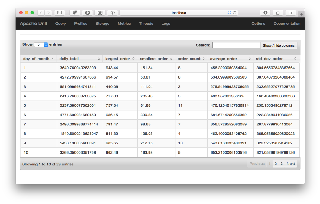
Figure 4-5. Data aggregated by day
If you wanted to present this data, you could format the numbers with a currency symbol and round them to the nearest decimal place by using the TO_NUMBER() function.
One major difference between Drill and relational databases is that Drill does not support column aliases in the GROUP BY clause. Thus, the following query would fail:
SELECTYEAR(date_field)ASyear_field,COUNT(*)FROMdfs.drill_tutorial.`data.csv`GROUPBYyear_field
To correct this you would simply need to replace GROUP BY year_field with GROUP BY YEAR(date_field).
Beware of Incorrect Column Names
If you include a field in the SELECT clause of a query that does not exist in your data, Drill will create an empty nullable INT column instead of throwing an error.
Other analytic functions: Window functions
In addition to the simple aggregate functions, Drill has a series of analytic functions known as window functions, which you can use to split the data and perform some operations on those sections. Although the window functions are similar to the aggregate functions used in a GROUP BY query, there is a difference in that window functions do not alter the number of rows returned. In addition to aggregating data, these functions are very useful for calculating metrics that relate to other rows, such as percentiles, rankings, and row numbers that do not necessarily need aggregation.
The basic structure of a query using a window function is as follows:
SELECTfields,FUNCTION(field)OVER(PARTITIONBYfieldORDERBYfield(Optional))
The PARTITION BY clause might look unfamiliar to you, but this is where you define the window or segment of the data upon which the aggregate function will operate.
In addition to AVG(), COUNT(), MAX(), MIN(), and SUM(), Drill includes several other window functions, as shown in Table 4-11.
| Function | Return type | Description |
|---|---|---|
|
|
|
Calculates the relative rank of the current row within the window: rows preceding/total rows. |
|
|
|
Returns the rank of the row within the window. Does not create gaps in the event of duplicate values. |
|
|
Same as input |
Returns the first value in the window. |
|
|
Same as input |
Returns the value after the current value in the window, |
|
|
Same as input |
Returns the last value in the window. |
|
|
Same as input |
Returns the value prior to the current value in the window, or |
|
|
|
Divides the rows for each window into a number of ranked groups. Requires the |
|
|
|
Calculates the percent rank of the current row within the window: (rank – 1) / (rows – 1). |
|
|
|
Similar to |
|
|
|
Returns the number of the row within the window. |
Comparison of aggregate and window analytic functions
The GitHub repository for this book contains a file called student_data.csvh, which contains some notional test scores from 10 different students. If you wanted to find each student’s average test score you could use either GROUP BY or window functions, but the GROUP BY option would be a simpler query. The following query accomplishes this task:
SELECTstudentID,AVG(CAST(scoreASFLOAT))ASaverage_score,MIN(CAST(scoreASFLOAT))ASmin_score,MAX(CAST(scoreASFLOAT))ASmax_scoreFROMdfs.drill_tutorial.`student_data.csvh`GROUPBYstudentID
Figure 4-6 demonstrates that this query produces the desired result.
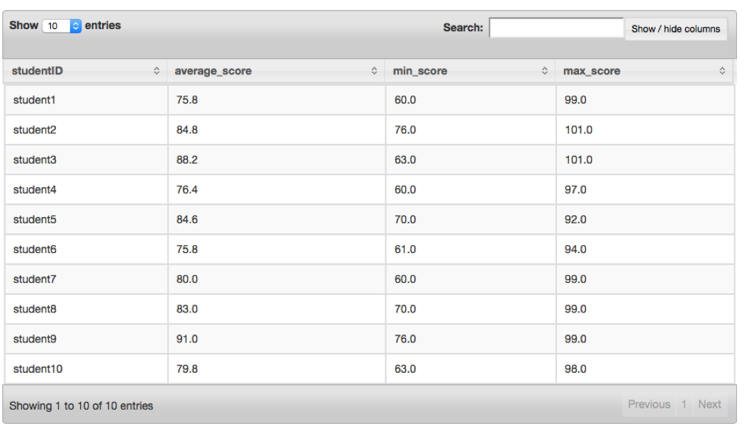
Figure 4-6. Aggregate query result
You could accomplish the same thing using window functions by using the following query:
SELECTDISTINCTstudentID,AVG(CAST(scoreASFLOAT))OVER(PARTITIONBYstudentID)ASavg_score,MIN(CAST(scoreASFLOAT))OVER(PARTITIONBYstudentID)ASmin_score,MAX(CAST(scoreASFLOAT))OVER(PARTITIONBYstudentID)ASmax_scoreFROMdfs.drill_tutorial.`student_data.csvh`
Note that you must use the DISTINCT keyword; otherwise, you will get duplicate rows. If you are working with large datasets, it is useful to be aware of the different methods of summarizing datasets because one might perform better on your data than the other.
Another example would be ranking each student’s score per test and calculating their quartile. In this example, it is not possible to do this using GROUP BY, so we must use the window functions RANK() and NTILE(). The following query demonstrates how to do this:
SELECTstudentID,testnumber,score,RANK()OVER(PARTITIONBYtestnumberORDERBYCAST(scoreASFLOAT)DESC)ASranking,NTILE(4)OVER(PARTITIONBYtestnumber)ASquartileFROMdfs.drill_tutorial.`student_data.csvh`
Figure 4-7 presents the results of this query.
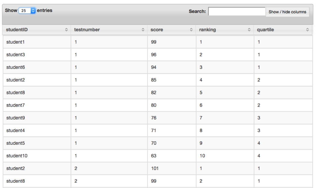
Figure 4-7. Window query results
You cannot use the results from window functions directly in a WHERE clause; thus, if you want to filter results from a window function, you must place the original query in a subquery, as shown here:
SELECT*FROM(SELECTstudentID,testnumber,score,RANK()OVER(PARTITIONBYtestnumberORDERBYCAST(scoreASFLOAT)DESC)ASranking,NTILE(4)OVER(PARTITIONBYtestnumber)ASquartileFROMdfs.drill_tutorial.`student_data.csvh`)ASstudent_dataWHEREstudent_data.quartile<=2
Figure 4-8 illustrates what this query returns.
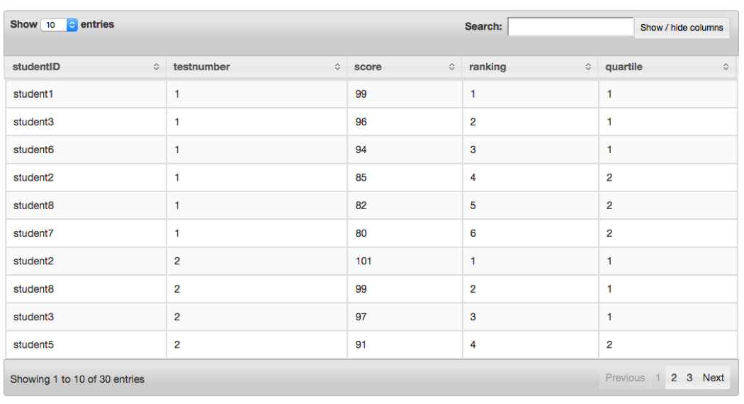
Figure 4-8. Window query results with filter
Common Problems in Querying Delimited Data
Because Drill allows you to query raw delimited data, it is quite likely that you will encounter certain problems along the way. We’ll look at how Drill processes data in more detail in Chapter 8, but for now, a little understanding of Drill can help you quickly get around these problems.
Spaces in Column Names
If your data has spaces or other reserved characters in a column name, or the column name itself is a reserved word, this will present a problem for Drill when you try to use the column name in a query. The easiest solution for this problem is to enclose all the column names in backticks (`) throughout your query.
For instance, this query will throw an error:
SELECTcustomername,dobFROMdfs.`customers.csv`
This query will not:
SELECT`customer name`,`dob`FROMdfs.`customers.csv`
Sometimes, columns can have spaces at the end of the field name. Enclosing the field name in backticks can solve this problem, as well—for example:
SELECT`field_1 `FROM...
Illegal Characters in Column Headers
We encountered this problem a while ago, and it took quite some time to diagnose. Essentially, we were querying a series of CSV files, and although we could query the files using SELECT * or most of the field names, the field we were interested in happened to be the last field in the row. When we tried to query that field specifically, we got an index out of bounds exception.
The reason for the error was that some of the CSV files were saved on a Windows machine, which encodes new lines with both a carriage return character (\r) and a newline character (\n), whereas Macs and Linux-based systems encode line endings with just the newline character (\n). In practice, what this meant was that the last field had an extra character in the field name; when we tried to query it without that character, Drill couldn’t find the field and threw an exception.
The easiest solution is to make sure that all your files are encoded using the Mac/Linux standard; that way, you won’t have any such problems.
Reserved Words in Column Names
A rather insidious problem that can bite you if you are not careful is when your data or column aliases are Drill reserved words.5 Often, you will have a data file that has a column called year or date. Because both of these are reserved words, Drill will throw errors if you attempt to access these columns in a query.
The solution to this problem is twofold. First, be aware of the Drill reserved words list, and second, as with the other situations, if you enclose a field name in backticks it will allow you to use reserved words in the query. We recommend that if you have a data file with reserved words as column names, you should either rename them in the file or in the query with an AS clause. A good rule of thumb is to always use backticks around all column names.
Conclusion
In this chapter, you learned how to query basic delimited data and to use Drill’s vast array of analytic functions to clean, prepare, and summarize that data for further analysis. In Chapter 5, you’ll take your analysis to the next level and learn how to apply these skills to nested datasets in formats such as JSON and Parquet, and other advanced formats.
1 The label “dfs” is actually arbitrary, and you can rename it whatever you want it to be. We will cover this later in this chapter.
2 This data is also available on the US government’s open data website.
3 For more information, see Oracle’s documentation on the DateTimeFormatter class.
4 Complete documentation for views in Drill is available on the Drill website.
5 You can find the complete list of Drill reserved words at the Apache Drill website.
Get Learning Apache Drill now with the O’Reilly learning platform.
O’Reilly members experience books, live events, courses curated by job role, and more from O’Reilly and nearly 200 top publishers.

