Chapter 4. Performance and Scale
One of the more challenging tasks of a network architect is ensuring that a design put forth meets the end-to-end solution requirements. The first step is identifying all of the roles in an architecture. This could be as simple as defining the edge, core, aggregation, and access tiers in the network. Each role has a specific set of responsibilities in terms of functionality and requirements. To map a product to a role in an architecture, the product must meet or exceed the requirements and functionality required by each role for which it’s being considered. Thus, building an end-to-end solution is a bit like a long chain: it’s only as strong as the weakest link.
The most common method of trying to identify the product capabilities, performance, and scale are through datasheets or the vendor’s account team. However, the best method is actually testing going through a proof of concept or certification cycle. Build out all of the roles and products in the architecture and measure the end-to-end results; this method quickly flushes out any issues before moving into procurement and production.
This chapter walks through all of the performance and scaling considerations required to successfully map a product into a specific role in an end-to-end architecture. Attributes such as MAC address, host entries, and IPv4 prefixes will be clearly spelled out. Armed with this data, you will be able to easily map the Juniper QFX10000 Series into many different roles in your existing network.
Design Considerations
Before any good network architect jumps head first into performance and scaling requirements, he will need to make a list of design considerations. Each design consideration places an additional tax on the network that is beyond the scope of traditional performance and scaling requirements.
Juniper Architectures Versus Open Architectures
The other common design option is to weight the benefits of Juniper architectures with open architectures. The benefits of a Juniper architecture is that it has been designed specifically to enable turn-key functionality, but the downside is that it requires a certain set of products to operate. The other option is open architecture. The benefit to an open architecture is that it can be supported across a set of multiple vendors, but the downside is that you might lose some capabilities that are only available in the Juniper architectures.
Generally, it boils down to the size of the network. If you know that your network will never grow past a certain size and you’re procuring all of the hardware upfront, using a Juniper architecture might simply outweigh all of the benefits of an open architecture, because there isn’t a need to support multiple vendors.
Another scenario is that your network is large enough that you can’t build it all at once and want a pay-as-you-grow option over the next five years. A logical option would be to implement open architectures so that as you build out your network, you aren’t limited in the number of options going forward. Another option would be to take a hybrid approach and build out the network in points of delivery (POD). Each POD could have the option to take advantage of proprietary architectures or not.
Each business and network are going to have any number of external forces that weigh on the decision to go with Juniper architectures or open architectures; more often than not, these decisions change over time. Unless you know 100 percent of these nuances up front, it’s important to select a networking platform that offers both Juniper architectures and open architectures.
The Juniper QFX10000 Series offers the best of both worlds. It equally supports Juniper architectures as well as open architectures:
- Juniper architectures
- The Juniper QFX10000 supports a plug-and-play Ethernet and fabric called Junos Fusion for Data Center (JFDC), which offers a single point of management for a topology of up to 64 top-of-rack (ToR) switches. JFDC allows for simple software upgrades one switch at a time, because it’s based on simple protocols such as IEEE 802.1BR and JSON.
- Open architectures
- The Juniper QFX10000 supports Ethernet VPN (EVPN)-Virtual Extensible LAN (VXLAN), which is quickly gaining traction as the de facto “open Ethernet fabric.” It also supports Multichassis Link Aggregation (MC-LAG) so that downstream devices can simply use IEEE 802.1AX Link Aggregation Control Protocol (LACP) to connect and transport data. The Juniper QFX10000 also supports a wide range of open protocols such as Border Gateway Protocol (BGP), Open Shortest Path First (OSPF), Intermediate System to Intermediate System (IS-IS), and a suite of Multiprotocol Label Switching (MPLS) technologies.
The Juniper QFX10000 makes a great choice no matter where you place it in your network. You could choose to deploy an open architecture today and then change to a Juniper architecture in the future. One of the best tools in creating a winning strategy is to keep the number of options high.
Performance
With the critical design considerations out of the way, now it’s time to focus on the performance characteristics of the Juniper QFX10000 series. Previously, in Chapter 1, we explored the Juniper Q5 chipset and how the Packet Forwarding Engine (PFE) and Switch Interface Board (SIB) work together in a balancing act of port density versus performance. Performance can be portrayed through two major measurements: throughput and latency. Let’s take a closer look at each.
Throughput
RFC 2544 was used as a foundation for the throughput testing. The test packet sizes ranged from 64 to 9,216 bytes, as shown in Figure 4-1. Both IPv4 and IPv6 traffic was used during the testing, and the results are nearly identical, so I displayed them as a single line. L2, L3, and VXLAN traffic was used during these tests.
The Juniper QFX10000 supports line-rate processing for packets above 144 bytes. 64 byte packets are roughly processed at 50 percent; as you work your way up to 100 bytes, they’re processed around 80 percent. At 144 bytes, the Juniper QFX10000 supports line-rate.
When it comes to designing an application-specific integrated circuit (ASIC), there are three main trade-offs: packet processing, power, and data path (buffering and scheduling). To create the Juniper Q5 chip with large buffers, high logical scale, and lots of features, a design trade-off had to be made. It was either increase the power, decrease the logical scale, reduce the buffer, or reduce the packet processing. Given the use cases for the data center, it’s common to not operate at full line-rate for packets under 200 bytes. You can see this design decision across all vendors and chipsets. Reducing packet processing for packets under 144 bytes was an easy decision, given that the majority of use cases do not require it; thus, the Juniper Q5 chip gets to take full advantage of low power, high scale, lots of features, and large buffer.

Figure 4-1. Graph showing Juniper QFX10002-72Q throughput versus packet size, tested at 5,760Gbps
Note
To learn more detailed test reports regarding EVPN-VXLAN, check out NetworkTest’s results. Big thanks to Michael Pergament for organizing the EVPN-VXLAN test results.
The data-plane encapsulation is also important to consider when measuring throughput. The following scenarios are very common in the data center:
-
Switching Ethernet frames
-
Routing IP packets
-
Encapsulating VXLAN headers
-
Switching MPLS labels
-
IPv4 versus IPv6
Each data-plane encapsulation requires different packet processing and lookups. The throughput graph in Figure 4-1 is an aggregate of IPv4, IPv6, switching, routing, MPLS, and VXLAN. The results were identical and so I combined them into a single throughput line. The Juniper Q5 chip has enough packet processing to handle a wide variety of data-plane encapsulations and actions (logging, policers, and filters) that it can handle five actions per packet without a drop in performance.
Latency
Latency is defined as the amount of time the network device takes to process a packet between ingress and egress port. The Juniper QFX10000 series has two ways to measure latency: within the same PFE, and between PFEs. If it’s within the same PFE, the latency is roughly 2.5 μs. If it’s between PFEs, it’s roughly 5.5 μs. There’s also a lot of variance between packet size and port speed. Check out Figure 4-2 for more detail.

Figure 4-2. Graph showing Juniper QFX10002-72Q latency versus packet size for 100/40/10GbE, tested at line-rate
The tests performed for Figure 4-2 were done between PFEs, which is the worst-case scenario. For example, it would be between port et-0/0/0 and et-0/0/71 which are located on different PFEs.
Logical Scale
Knowing the logical scale for a particular platform is crucial for understanding how well it can perform in a specific role in an overall network architecture. Most often, it requires you invest a lot of time testing the platform to really understand the details of the platform.
One caveat to logical scale is that it’s always a moving target between software releases. Although the underlying hardware might be capable of more scale, the software must fully support and utilize it. Some logical scale is limited by physical constraints such as the number of ports. For example, the Juniper QFX10002-72Q supports only 144 aggregated interfaces. This seems like a very low number until you realize that the maximum number of 10GbE interfaces is 288; and if you bundle all of the interfaces with two members each, it’s a total of 144 aggregated interfaces.
Table 4-1 takes a closer look at the logical scale as of the Juniper QFX10002-72Q running Junos 15.1X53D10.
| Attribute | Result |
|---|---|
| VLAN | 4,093 |
| RVI | 4,093 |
| Aggregated interfaces | 144 |
| Subinterfaces | 16,000 |
| vMembers | 32,000 per PFE |
| MSTP instances | 64 |
| VSTP instances | 510 |
| PACL ingress terms | 64,000 |
| PACL egress filters | 64,000 |
| VACL ingress filters | 4,093 |
| VACL egress terms | 4,093 |
| VACL ingress filters | 64,000 |
| VACL egress filters | 64,000 |
| RACL ingress filters | 10,000 |
| RACL egress filters | 10,000 |
| RACL ingress terms | 64,000 |
| RACL egress terms | 64,000 |
| PACL policers | 8,192 |
| VACL policers | 8,192 |
| RACL policers | 8,192 |
| Firewall counters | 64,000 |
| BGP neighbors | 4,000 |
| OSPF adjacencies | 1,000 |
| OSPF areas | 500 |
| VRRP instances | 2,000 |
| BFD clients | 1,000 |
| VRFs | 4,000 |
| RSVP ingress LSPs | 16,000 |
| RSVP egress LSPs | 16,000 |
| RSVP transit LSPs | 32,000 |
| LDP sessions | 1,000 |
| LDP labels | 115,000 |
| GRE tunnels | 4,000 |
| ECMP | 64-way |
| ARP—per PFE | 64,000 |
| MAC—per PFE | 96,000 |
| IPv4 FIB | 256,000/2,000,000 |
| IPv6 FIB | 256,000/2,000,000 |
| IPv4 hosts | 2,000,000 |
| IPv6 hosts | 2,000,000 |
| IPv4 RIB | 10,000,000 |
| IPv6 RIB | 4,000,000 |
Some attributes are global maximums, whereas others are listed as per PFE. There are features such as MAC address learning and Access Control Lists (ACLs) that can be locally significant and applied per PFE. For example, if you install MAC address 00:00:00:00:00:AA on PFE-1, there’s no need to install it on PFE-2, unless it’s part of an aggregated interface. For attributes that are per PFE, you can just multiply that value by the number of PFEs in a system to calculate the global maximum. For example, the Juniper QFX10002-72Q has six PFEs, so you can multiply 6 for the number of MAC addresses, which is 576,000 globally.
Warning
Be aware that Table 4-1 shows the logical scale for the Juniper QFX10002-72Q based on Junos 15.1X53D10. Keep in mind that these scale numbers will change between software releases and improve over time.
Firewall Filter Usage
One of the more interesting scaling attributes are firewall filters, which you can apply anywhere within the system. Such filters could be per port, which would limit the network state to a particular ASIC within the system. You could apply other firewall filters to a VLAN, which would spread the firewall filter state across every single ASIC within the system. Over time, firewall filters will grow in size and scope; ultimately, there will exist state fragmentation on the switch, by the nature and scope of the firewall filters.
One common question is “How do you gauge how many system resources are being used by the firewall filters?” There’s no easy way to do this directly in the Junos command line; it requires that you drop to the microkernel and perform some low-level commands to get hardware summaries.
Dropping to the microkernel is different depending on what platform you’re using. For the Juniper QFX100002, it’s fairly straightforward because there’s a single FPC: FPC0. However, if you’re using a Juniper QFX10008 or QFX10016, you’ll need to log in to each line card separately to look at the hardware state.
In our example, we’ll use a Juniper QFX10002-72Q. Let’s drop into the shell:
{master:0}
root@st-v44-pdt-elite-01> start shell
root@st-v44-pdt-elite-01:~ # vty fpc0


TOR platform (2499 Mhz Pentium processor, 2047MB memory, 0KB flash)

TFXPC0(vty)#
The next step is to use the show filter hw summary command:
TFXPC0(vty)# show filter hw sum

  Chip Instance: 0

  HW Resource    Capacity          Used          Available
  ---------------------------------------------------------
  Filters         8191                2            8189
  Terms           65536              69           65467

  Chip Instance: 1

  HW Resource    Capacity          Used          Available
  ---------------------------------------------------------
  Filters         8191                2            8189
  Terms           65536              69           65467

  Chip Instance: 2

  HW Resource    Capacity          Used          Available
  ---------------------------------------------------------
  Filters         8191                2            8189
  Terms           65536              69           65467

  Chip Instance: 3

  HW Resource    Capacity          Used          Available
  ---------------------------------------------------------
  Filters         8191                2            8189
  Terms           65536              69           65467

  Chip Instance: 4

  HW Resource    Capacity          Used          Available
  ---------------------------------------------------------
  Filters         8191                2            8189
  Terms           65536              69           65467

  Chip Instance: 5

  HW Resource    Capacity          Used          Available
  ---------------------------------------------------------
  Filters         8191                2            8189
  Terms           65536              69           65467
The hardware resources are summarized by each PFE. In the case of the Juniper QFX10002-72Q, there are six ASICs. Firewall filters are broken down by the number of actual filters and the number of terms within. Each PFE on the Juniper QFX10000 can support 8,192 filters and 65,536 terms. These available allocations are global and must be shared for both ingress and egress filters.
I have created a simple firewall filter and applied it across an entire VLAN that has port memberships across every ASIC in the switch. Let’s run the command and see how the allocations have changed:
TFXPC0(vty)# show filter hw sum

  Chip Instance: 0

  HW Resource    Capacity          Used          Available
  ---------------------------------------------------------
  Filters         8191                3            8188
  Terms           65536              71           65465

  Chip Instance: 1

  HW Resource    Capacity          Used          Available
  ---------------------------------------------------------
  Filters         8191                3            8188
  Terms           65536              71           65465

  Chip Instance: 2

  HW Resource    Capacity          Used          Available
  ---------------------------------------------------------
  Filters         8191                3            8188
  Terms           65536              71           65465

  Chip Instance: 3

  HW Resource    Capacity          Used          Available
  ---------------------------------------------------------
  Filters         8191                3            8188
  Terms           65536              71           65465

  Chip Instance: 4

  HW Resource    Capacity          Used          Available
  ---------------------------------------------------------
  Filters         8191                3            8188
  Terms           65536              71           65465

  Chip Instance: 5

  HW Resource    Capacity          Used          Available
  ---------------------------------------------------------
  Filters         8191                3            8188
  Terms           65536              71           65465
The new VLAN filter has used a single filter and two term allocations on each ASIC within the system. However, if you created a simple firewall filter and applied it to only an interface, you would see allocations being used on a single ASIC.
Hashing
There are two types of hashing on the Juniper QFX10000 Series: static and adaptive. Static hashing is basically the type of hashing you are already familiar with: the switch looks at various fields in the packet header and makes a decision as to which interface to forward it. Adaptive hashing is a little bit different; it incorporates the packets per second (pps) or bits per second (bps) to ensure that new flows are not hashed to over-utilized links. The goal of adaptive hashing is to have all links in an aggregated Ethernet (AE) bundle being used equally over time.
Static
Every time you create an AE bundle in Junos, it internally allocates 256 buckets per AE. The buckets are equally divided across the number of member links. For example, if ae0 has 4 links, each member would be assigned 64 buckets each, as shown in Figure 4-3.

Figure 4-3. Static hashing on an interface bundle with four members
The number of buckets has no special meaning; it’s just an arbitrary number that aligns well with Juniper’s hashing algorithm. What matters is the distribution of buckets across the member interfaces. When all member interfaces are up and forwarding traffic, the number of buckets is equally distributed across each member interface. However, if there is a link failure, the number of buckets is redistributed to the remaining number of member interfaces. For example, if there were a single link failure in Figure 4-3, the three remaining links would receive 85, 85, and 86 buckets, respectively. When the failed link comes back up, the number of buckets assigned to each member interface would revert back to 64.
At a high level, ingress packets are inspected for interesting bits, which are passed on to the hash function, as depicted in Figure 4-4. The hash function takes the interesting bits as an input and outputs a number between 0 and 255, which corresponds to a bucket number. Also in the figure, the hash function decided to use bucket 224, which is currently owned by member interface xe-0/0/3. As soon as the ingress packet is mapped to a specific bucket, the traffic is forwarded to the corresponding interface.

Figure 4-4. How ingress packets are mapped to buckets and forwarded within AE bundles
Adaptive
Adaptive load balancing uses the same bucket architecture as static hashing; however, the big difference is that adaptive can change bucket allocations on the fly. There are two stages with adaptive load balancing: calculation and adjustment. You can think of the calculation phase as a scan interval. Every so often the AE bundle will look at all of the member links and evaluate the amount of traffic flowing through each. The adjustment phase changes the bucket allocations so that member links with a lot of traffic can back off, and under-utilized member links can take additional load. The intent is for each member of the AE bundle to have an equal amount of traffic.
The traffic can be measured at each scan interval in two different ways: pps or bps. Depending on the use case of the AE bundle, pps and bps play a large role. For example, if you’re a company that processes a lot of small web queries that are fairly static in nature, using pps might make more sense because it’s transaction oriented. On the other hand, if you’re handling transit traffic and have no control of the flows, bps will make more sense.
Take, for example, an AE bundle with four links, as illustrated in Figure 4-5. During the calculation phase, the AE bundle inspects the pps of each member link. If the pps isn’t within a specific threshold, the AE bundle will adjust the bucket allocation so that under-utilized links will attract more hash functions and over-utilized links will attract less hash functions.
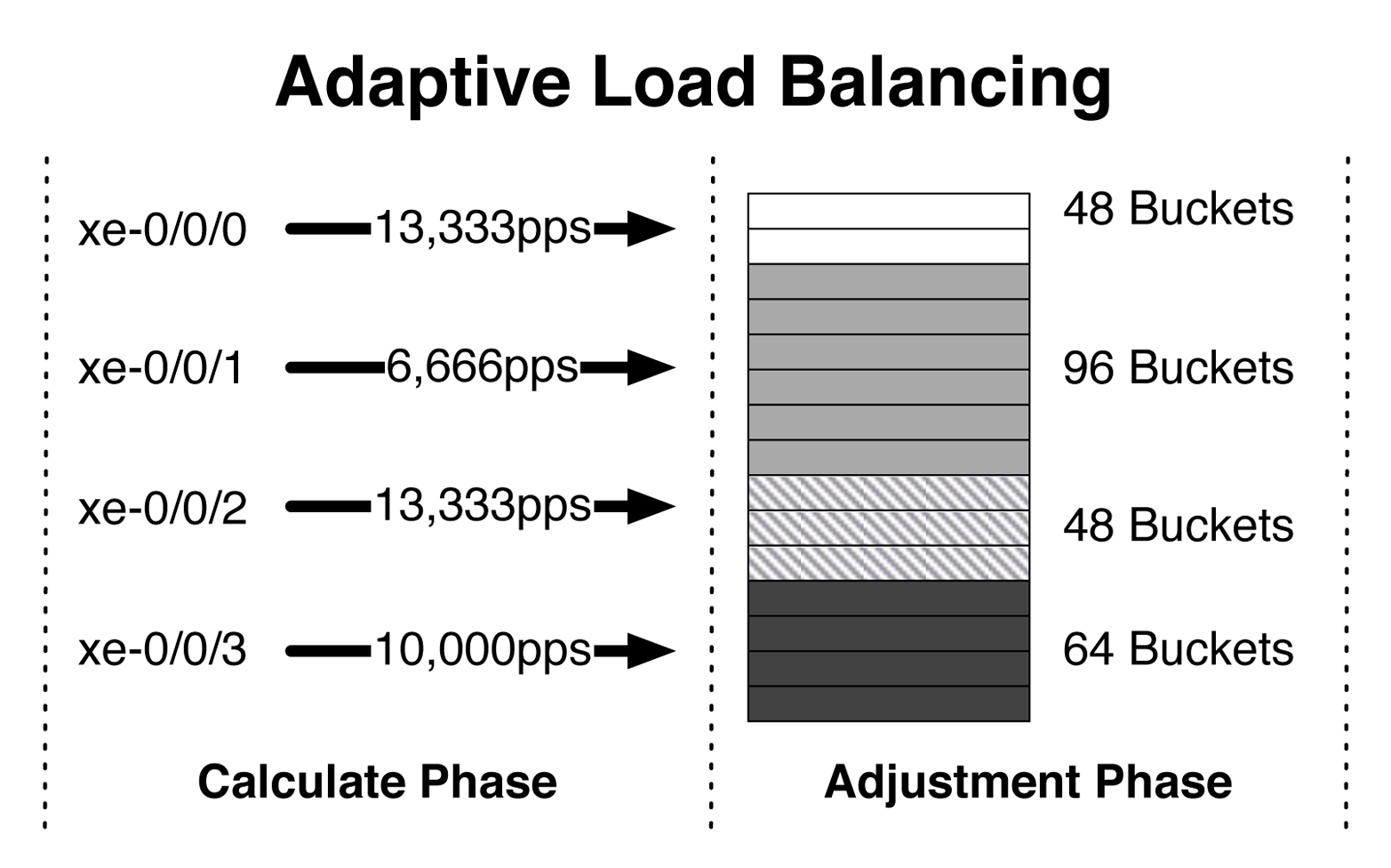
Figure 4-5. Adaptive load balancing
For example, in the figure, interface xe-0/0/0 and xe-0/0/2 are handling 13,333 pps, whereas xe-0/0/1 is only at 6,666 pps. The AE bundle reduces the number of bucket allocations for both xe-0/0/0 and xe-0/0/2 and increases the bucket allocations for xe-0/0/1. The intent is to even out the pps across all four interfaces. A single calculation phase isn’t enough to correct the entire AE bundle, and multiple scans are required over time to even things out.
Adaptive load balancing can be enabled on a per AE basis (Figure 4-6). In other words, you can have a set of AE interfaces that are a normal static LAG and another set of AE interfaces that are enabled for adaptive load balancing.
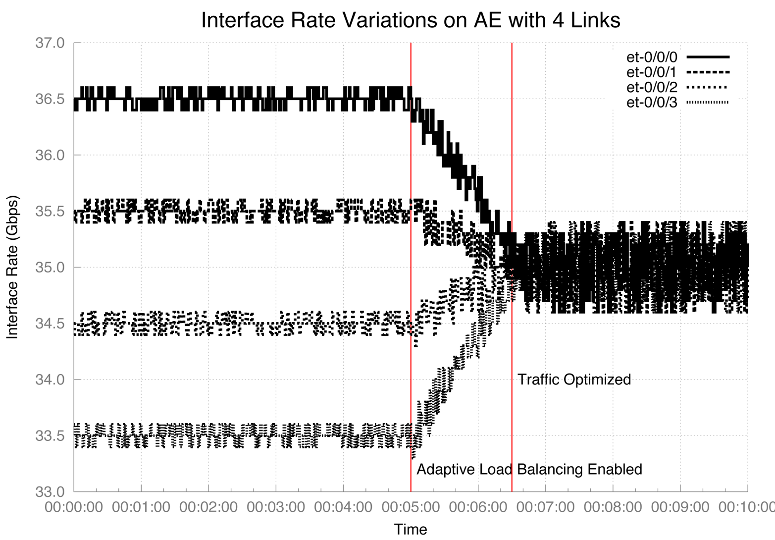
Figure 4-6. Adaptive load balancing enabled on an AE bundle
Configuration
Now that you understand more about adaptive load balancing, let’s take a look at how to configure it. You’ll find the new knob under aggregated-ether-options:
dhanks@QFX10002# set interfaces ae0 aggregated-ether-options load-balance adaptive ?
Possible completions:
  enable               Enable
  tolerance            Tolerance in percentage (1..100, default 20percent)
  scan-interval        Scan interval in seconds (10..600, default 30sec)
  criterion             pps or bps (default bps)
There are four new options: enable, tolerance, scan-interval, and criterion. You must set the enable knob for it to work. The tolerance sets the percentage of variance between flows; by default, it’s set to 20 percent. The smaller the tolerance, the better it balances better bandwidth, but it takes longer.
The scan-interval sets the frequency at which the AE interface performs the calculation phase and recalculates the bucket allocations. By default, it’s set to 30 seconds. The final option is the criterion, with which you can select pps or bps; by default, it’s bps.
dhanks@QFX10002> show interfaces ae0 extensive
Physical interface: ae0, Enabled, Physical link is Up
<truncated>
  Logical interface ae0.0
<truncated>
    Adaptive Statistics:
        Adaptive Adjusts  :        264
        Adaptive Scans    :     172340
        Adaptive Tolerance:         20%
        Adaptive Updates  :         20
You can use the show interfaces command with the extensive knob to get all the gory details about adaptive load balancing. You can see how many adjustments it made to the buckets, how many times it has scanned the particular interface, and how many times it has been updated.
Forwarding Options
When it comes to hashing, the Juniper QFX10000 Series has a lot of different options for various types of data-plane encapsulations. Table 4-2 lists these options.
| Attributes | Field Bits | L2 | IPv4 | IPv6 | MPLS |
|---|---|---|---|---|---|
| Source MAC | 0–47 | O | O | O | O |
| Destination MAC | 0–47 | O | O | O | O |
| EtherType | 0–15 | D | D | D | D |
| VLAN ID | 0–11 | D | D | D | D |
| GRE/VXLAN | Varies | O | O | O | O |
| Source IP | 0–31 | D | D | D | |
| Destination IP | 0–31 | D | D | D | |
| Ingress interface | D | D | D | D | |
| Source port | 0–15 | D | D | D | |
| Destination port | 0–15 | D | D | D | |
| IPv6 flow label | 0–19 | D | D | ||
| MPLS | D |
In Table 4-2, “O” stands for optional, and “D” for default. So, whenever you see a default setting, that’s just how the Juniper QFX10000 works out of the box. If you want to add additional bits into the hash function, you can selectively enable them per data-plane encapsulation if it’s listed as “O.”
Summary
This chapter has covered the major design decisions between Juniper architectures and open architectures. Juniper architectures allow for ease of use at the expense of only working with Juniper switches. The open architectures make it possible for any other vendor to participate with open protocols, but sometimes at the expense of features. We also reviewed the performance in terms of throughput and latency. The Juniper QFX10000 operates at line rate above 144 byte packets while performing any data-plane encapsulation, deep buffering, and high logical scale. Next, we took a look at the logical scale of the QFX10002-72Q with Junos 15.1X53D10. We wrapped up the chapter with a review on how the Juniper QFX10000 handles static and adaptive hashing.
Chapter Review Questions
-
Which is a Juniper architecture?
-
MC-LAG
-
Junos Fusion
-
MP-BGP
-
EVPN-VXLAN
-
-
The Juniper QFX10002-72Q is line-rate after what packet size?
-
64B
-
128B
-
144B
-
200B
-
-
Juniper QFX10002-72Q supports 1 M IPv4 entries in the FIB. What about IPv6?
-
Only half the amount of IPv4
-
Only a quarter amount of IPv4
-
The same as IPv4
-
-
Why does the Juniper QFX10002-72Q support only 144 AE interfaces?
-
Kernel limitations
-
Not enough CPU
-
Physical port limitations
-
Not enough memory
-
-
How do you set the threshold between flows for adaptive load balancing?
-
scan-interval -
enable -
tolerance -
buckets
-
Chapter Review Answers
-
Answer: A and B. MC-LAG is a little tricky; it depends how you view it. From the perspective of the CE, it works with any other device in the network. However, between PE switches, it must be a Juniper device for ICCP to work. Junos Fusion for Data Center requires the Juniper QFX10000 as the aggregation device and Juniper top-of-rack switches for the satellite devices.
-
Answer: C. The Juniper QFX10002-72Q is line-rate for packets over 144 bytes.
-
Answer: C. The Juniper QFX10002-72Q supports 1M entries in the FIB for both IPv4 and IPv6 at the same time.
-
Answer: C. The Juniper QFX10002-72Q had a maximum of 288x10GbE interfaces. If you pair of every single 10GbE interface, that is a total of 144 AE interfaces. It’s purely a physical port limitation.
-
Answer: C. Adaptive load balancing can adjust the variance between flows with the
toleranceknob.
Get Juniper QFX10000 Series now with the O’Reilly learning platform.
O’Reilly members experience books, live events, courses curated by job role, and more from O’Reilly and nearly 200 top publishers.

