Chapter 9. Optimizing
One reason you might be reading this book in the first place is that you don’t just want pretty graphics; you want fast graphics. Since OpenGL ES gives you the lowest possible level of access to Apple’s graphics hardware, it’s the ideal API when speed is your primary concern. Many speed-hungry developers use OpenGL even for 2D games for this reason.
Until this point in this book, we’ve been focusing mostly on the fundamentals of OpenGL or showing how to use it to achieve cool effects. We’ve mentioned a few performance tips along the way, but we haven’t dealt with performance head-on.
Instruments
Of all the performance metrics, your
frame rate (number of
presentRenderbuffer calls per second) is the metric
that you’ll want to measure most often. We presented one way of
determining frame rate in Chapter 7, where we rendered an
FPS counter on top of the scene. This was convenient and simple, but
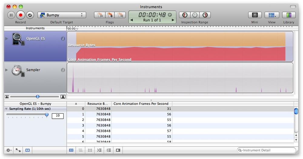
Apple’s Instruments tool (Figure 9-1) can accomplish the same thing, and much
more—without requiring you to modify your application!
The best part is that it’s included in the SDK that you
already have.
Warning
As with any performance analysis tool, beware of the Heisenberg effect. In this context, I’m referring to the fact that measuring performance can, in itself, affect performance. This has never been problematic for me, and it’s certainly not as bothersome as a Heisenbug (a bug that seems to vanish when you’re in the debugger).
First, be sure that your Active SDK (upper-left corner of Xcode) is set to a Device configuration rather than a Simulator configuration. Next, click the Run menu, and select the Run with Performance Tool submenu. You should see an option for OpenGL ES (if not, you probably have your SDK set to Simulator).
While your application is running, Instruments is constantly updating an EKG-like graph of your frame rate and various other metrics you may be interested in. Try clicking the information icon in the OpenGL ES panel on the left, and then click the Configure button. This allows you to pick and choose from a slew of performance metrics.
Instruments is a great tool for many aspects of performance analysis, not just OpenGL. I find that it’s particularly useful for detecting memory leaks. The documentation for Instruments is available on the iPhone developer site. I encourage you to read up on it and give it a whirl, even if you’re not experiencing any obvious performance issues.
Understand the CPU/GPU Split
Don’t forget that the bottleneck of your application may be on the CPU side rather than in the graphics processing unit (GPU). You can determine this by diving into your rendering code and commenting out all the OpenGL function calls. Rerun your app with Instruments, and observe the frame rate; if it’s unchanged, then the bottleneck is on the CPU. Dealing with such bottlenecks is beyond the scope of this book, but Instruments can help you track them down. Keep in mind that some types of CPU work (such as transforming vertices) can be moved to the GPU through clever usage of OpenGL.
Vertex Submission: Above and Beyond VBOs
The manner in which you submit vertex data to OpenGL ES can have a huge impact on performance. The most obvious tip is something I mentioned early in this book: use vertex buffer objects whenever possible. They eliminate costly memory transfers. VBOs don’t help as much with older devices, but using them is a good habit to get into.
Batch, Batch, Batch
VBO usage is just the tip of the iceberg. Another best practice that you’ll hear a lot about is draw call batching. The idea is simple: try to render as much as possible in as few draw calls as possible. Consider how you’d go about drawing a human head. Perhaps your initial code does something like Example 9-1.
glBindTexture(...);  // Bind the skin texture.
glDrawArrays(...);   // Render the head.
glDrawArrays(...);   // Render the nose.
glLoadMatrixfv(...); // Shift the model-view to the left side.
glDrawArrays(...);   // Render the left ear.

glBindTexture(...);  // Bind the eyeball texture.
glDrawArrays(...);   // Render the left eye.
glLoadMatrixfv(...); // Shift the model-view to the right side.

glBindTexture(...);  // Bind the skin texture.
glDrawArrays(...);   // Render the right ear.

glBindTexture(...);  // Bind the eyeball texture.
glDrawArrays(...);   // Render the right eye.
glLoadMatrixfv(...); // Shift the model-view to the center.

glBindTexture(...);  // Bind the lips texture.
glDrawArrays(...);   // Render the lips.
Right off the bat, you should notice that the head and nose can be “batched” into a single VBO. You can also do a bit of rearranging to reduce the number of texture binding operations. Example 9-2 shows the result after this tuning.
glBindTexture(...);  // Bind the skin texture.
glDrawArrays(...);   // Render the head and nose.
glLoadMatrixfv(...); // Shift the model-view to the left side.
glDrawArrays(...);   // Render the left ear.
glLoadMatrixfv(...); // Shift the model-view to the right side.
glDrawArrays(...);   // Render the right ear.

glBindTexture(...);  // Bind the eyeball texture.
glLoadMatrixfv(...); // Shift the model-view to the left side.
glDrawArrays(...);   // Render the left eye.
glLoadMatrixfv(...); // Shift the model-view to the left side.
glDrawArrays(...);   // Render the right eye.
glLoadMatrixfv(...); // Shift the model-view to the center.

glBindTexture(...);  // Bind the lips texture.
glDrawArrays(...);   // Render the lips.
Try combing through the code again to see whether anything can be eliminated. Sure, you might be saving a little bit of memory by using a single VBO to represent the ear, but suppose it’s a rather small VBO. If you add two instances of the ear geometry to your existing “head and nose” VBO, you can eliminate the need for changing the model-view matrix, plus you can use fewer draw calls. Similar guidance applies to the eyeballs. Example 9-3 shows the result.
You’re not done yet. Remember texture atlases, first presented in Animation with Sprite Sheets? By tweaking your texture coordinates and combining the skin texture with the eye and lip textures, you can reduce the rendering code to only two lines:
glBindTexture(...);  // Bind the atlas texture.
glDrawArrays(...);   // Render the head and nose and ears and eyes and lips.
OK, I admit this example was rather contrived. Rarely does production code make linear sequences of OpenGL calls as I’ve done in these examples. Real-world code is usually organized into subroutines, with plenty of stuff going on between the draw calls. But, the same principles apply. From the GPU’s perspective, your application is merely a linear sequence of OpenGL calls. If you think about your code in this distilled manner, potential optimizations can be easier to spot.
Interleaved Vertex Attributes
You might hear the term interleaved data being thrown around in regard to OpenGL optimizations. It is indeed a good practice, but it’s actually nothing special. In fact, every sample in this book has been using interleaved data (for a diagram, flip back to Figure 1-8 in Chapter 1). Using our C++ vector library, much of this book’s sample code declares a plain old data (POD) structure representing a vertex, like this:
struct Vertex {
    vec3 Position;
    vec3 Normal;
    vec2 TexCoord;
};
When we create the VBO, we populate it with
an array of Vertex objects. When it comes time to
render the geometry, we usually do something like Example 9-4.
glBindBuffer(...);
GLsizei stride = sizeof(Vertex);

// ES 1.1
glVertexPointer(3, GL_FLOAT, stride, 0);
glNormalPointer(GL_FLOAT, stride, offsetof(Vertex, Normal));
glTexCoordPointer(2, GL_FLOAT, stride, offsetof(Vertex, TexCoord));

// ES 2.0
glVertexAttribPointer(positionAttrib, 3, GL_FLOAT, GL_FALSE, stride, 0);
glVertexAttribPointer(normalAttrib, 3, GL_FALSE,
                      GL_FALSE, stride, offsetof(Vertex, Normal));
glVertexAttribPointer(texCoordAttrib, 2, GL_FLOAT,
                      GL_FALSE, stride, offsetof(Vertex, TexCoord));
OpenGL does not require you to arrange VBOs in the previous manner. For example, consider a small VBO with only three vertices. Instead of arranging it like this:
Position-Normal-TexCoord-Position-Normal-TexCoord-Position-Normal-TexCoord
you could lay it out it like this:
Position-Position-Position-Normal-Normal-Normal-TexCoord-TexCoord-TexCoord
This is perfectly acceptable (but not advised); Example 9-5 shows the way you’d submit it to OpenGL.
glBindBuffer(...);

// ES 1.1
glVertexPointer(3, GL_FLOAT, sizeof(vec3), 0);
glNormalPointer(GL_FLOAT, sizeof(vec3), sizeof(vec3) * VertexCount);
glTexCoordPointer(2, GL_FLOAT, sizeof(vec2),
                  2 * sizeof(vec3) * VertexCount);

// ES 2.0
glVertexAttribPointer(positionAttrib, 3, GL_FLOAT,
                      GL_FALSE, sizeof(vec3), 0);
glVertexAttribPointer(normalAttrib, 3, GL_FALSE,
                      GL_FALSE, sizeof(vec3),
                      sizeof(vec3) * VertexCount);
glVertexAttribPointer(texCoordAttrib, 2, GL_FLOAT,
                      GL_FALSE, sizeof(vec2),
                      2 * sizeof(vec3) * VertexCount);
When you submit vertex data in this manner, you’re forcing the driver to reorder the data to make it amenable to the GPU.
Optimize Your Vertex Format
One aspect of vertex layout you might be wondering about is the ordering of attributes. With OpenGL ES 2.0 and newer Apple devices, the order has little or no impact on performance (assuming you’re using interleaved data). On first- and second-generation iPhones, Apple recommends the following order:
You might be wondering about the two “bone” attributes—stay tuned, well discuss them later in the chapter.
Another way of optimizing your vertex format is shrinking the size of the attribute types. In this book, we’ve been a bit sloppy by using 32-bit floats for just about everything. Don’t forget there are other types you can use. For example, floating point is often overkill for color, since colors usually don’t need as much precision as other attributes.
// ES 1.1
// Lazy iPhone developer:
glColorPointer(4, GL_FLOAT, sizeof(vertex), offset);

// Rock Star iPhone developer!
glColorPointer(4, GL_UNSIGNED_BYTE, sizeof(vertex), offset);

// ES 2.0
// Lazy:
glVertexAttribPointer(color, 4, GL_FLOAT, GL_FALSE, stride, offset);

// Rock star!
glVertexAttribPointer(color, 4, GL_UNSIGNED_BYTE,
                      GL_FALSE, stride, offset);
Warning
Don’t use GL_FIXED.
Because of the iPhone’s architecture, fixed-point numbers actually
require more processing than floating-point
numbers. Fixed-point is available only to comply with the Khronos
specification.
Apple recommends aligning vertex attributes in memory according to their native alignment. For example, a 4-byte float should be aligned on a 4-byte boundary. Sometimes you can deal with this by adding padding to your vertex format:
struct Vertex {
    vec3 Position;
    unsigned char Luminance;
    unsigned char Alpha;
    unsigned short Padding;
};
Use the Best Topology and Indexing
Apple’s general advice (at the time of this
writing) is to prefer GL_TRIANGLE_STRIP over
GL_TRIANGLES. Strips require fewer vertices but
usually at the cost of more draw calls. Sometimes you can reduce the
number of draw calls by introducing degenerate triangles into your
vertex buffer.
Strips versus separate triangles, indexed versus nonindexed; these all have trade-offs. You’ll find that many developers have strong opinions, and you’re welcome to review all the endless debates on the forums. In the end, experimentation is the only reliable way to determine the best tessellation strategy for your unique situation.
Imagination Technologies provides code for converting lists into strips. Look for PVRTTriStrip.cpp in the OpenGL ES 1.1 version of the PowerVR SDK (first discussed in Texture Compression with PVRTC). It also provides a sample app to show it off (Demos/OptimizeMesh).
Lighting Optimizations
If your app has highly tessellated geometry (lots of tiny triangles), then lighting can negatively impact performance. The following sections discuss ways to optimize lighting. Use your time wisely; don’t bother with these optimizations without first testing if you’re fill rate bound. Applications that are fill rate bound have their bottleneck in the rasterizer, and lighting optimizations don’t help much in those cases—unless, of course, the app is doing per-pixel lighting!
There’s a simple test you can use to determine
whether you’re fill rate bound. Try modifying the parameters to
glViewport to shrink your viewport to a small size. If
this causes a significant increase in your frame rate, you’re probably
fill rate bound.
If you discover that you’re neither fill rate bound nor CPU bound, the first thing to consider is simplifying your geometry. This means rendering a coarser scene using larger, fewer triangles. If you find you can’t do this without a huge loss in visual quality, consider one of the optimizations in the following sections.
Note
If you’re CPU bound, try turning off Thumb mode; it enables a special ARM instruction set that can slow you down. Turn it off in Xcode by switching to a Device configuration and going to Project→Edit Project Settings→Build Tab→Show All Settings, and uncheck the “Compile for Thumb” option under the Code Generation heading.
Object-Space Lighting
We briefly mentioned object-space lighting in Bump Mapping and DOT3 Lighting; to summarize, in certain circumstances, surface normals don’t need transformation when the light source is infinitely distant. This principle can be applied under OpenGL ES 1.1 (in which case the driver makes the optimization for you) or in OpenGL ES 2.0 (in which case you can make this optimization in your shader).
To specify an infinite light source, set the W component of your light position to zero. But what are those “certain circumstances” that we mentioned? Specifically, your model-view matrix cannot have non-uniform scale (scale that’s not the same for all three axes). To review the logic behind this, flip back to Normal Transforms Aren’t Normal.
DOT3 Lighting Revisited
If per-vertex lighting under OpenGL ES 1.1 causes performance issues with complex geometry or if it’s producing unattractive results with coarse geometry, I recommend that you consider DOT3 lighting. This technique leverages the texturing hardware to perform a crude version of per-pixel lighting. Refer to Normal Mapping with OpenGL ES 1.1 for more information.
Baked Lighting
The best way to speed up your lighting calculations is to not perform them at all! Scenes with light sources that don’t move can be prelit, or “baked in.” This can be accomplished by performing some offline processing to create a grayscale texture (also called a light map). This technique is especially useful when used in conjunction with multitexturing.
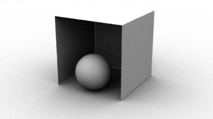
As an added benefit, baked lighting can be used to create a much higher-quality effect than standard OpenGL lighting. For example, by using a raytracing tool, you can account for the ambient light in the scene, producing beautiful soft shadows (see Figure 9-2). One popular offline tool for this is xNormal, developed by Santiago Orgaz.
Texturing Optimizations
If your frame rate soars when you try disabling texturing, take a look at the following list:
Don’t use textures that are any larger than necessary. This is especially true when porting a desktop game; the iPhone’s small screen usually means that you can use smaller textures.
Older devices have 24MB of texture memory; don’t exceed this. Newer devices have unified memory, so it’s less of a concern.
Another tip: it won’t help with frame rate, but
your load time might be improved by converting your image files into a
“raw” format like PVRTC or even into a C-array header file. You can do
either of these using
PVRTexTool (The PowerVR SDK and Low-Precision Textures).
Culling and Clipping
Avoid telling OpenGL to render things that aren’t visible anyway. Sounds easy, right? In practice, this guideline can be more difficult to follow than you might think.
Polygon Winding
Consider something simple: an OpenGL scene with a spinning, opaque sphere. All the triangles on the “front” of the sphere (the ones that face that camera) are visible, but the ones in the back are not. OpenGL doesn’t need to process the vertices on the back of the sphere. In the case of OpenGL ES 2.0, we’d like to skip running a vertex shader on back-facing triangles; with OpenGL ES 1.1, we’d like to skip transform and lighting operations on those triangles. Unfortunately, the graphics processor doesn’t know that those triangles are occluded until after it performs the rasterization step in the graphics pipeline.
So, we’d like to tell OpenGL to skip the back-facing vertices. Ideally we could do this without any CPU overhead, so changing the VBO at each frame is out of the question.
How can we know ahead of time that a triangle is back-facing? Consider a single layer of triangles in the sphere; see Figure 9-3. Note that the triangles have consistent “winding”; triangles that wind clockwise are back-facing, while triangles that wind counterclockwise are front-facing.
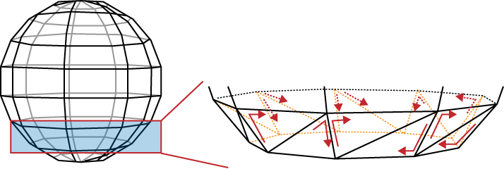
OpenGL can quickly determine whether a given triangle goes clockwise or counterclockwise. Behind the scenes, the GPU can take the cross product of two edges in screen space; if the resulting sign is positive, the triangle is front-facing; otherwise, it’s back-facing.
Face culling is enabled like so:
glEnable(GL_CULL_FACE);
You can also configure OpenGL to define which winding direction is the front:
glFrontFace(GL_CW);  // front faces go clockwise
glFrontFace(GL_CCW); // front faces go counterclockwise (default)
Depending on how your object is tessellated, you may need to play with this setting.
Use culling with caution; you won’t always want it to be enabled! It’s mostly useful for opaque, enclosed objects. For example, a ribbon shape would disappear if you tried to view it from the back.
As an aside, face culling is useful for much more than just performance optimizations. For example, developers have come up with tricks that use face culling in conjunction with the stencil buffer to perform CSG operations (composite solid geometry). This allows you to render shapes that are defined from the intersections of other shapes. It’s cool stuff, but we don’t go into it in detail in this book.
User Clip Planes
User clip planes provide another way of culling away unnecessary portions of a 3D scene, and they’re often useful outside the context of performance optimization. Here’s how you enable a clip plane with OpenGL ES 1.1:
void EnableClipPlane(vec3 normal, float offset)
{
    glEnable(GL_CLIP_PLANE0);
    GLfloat planeCoefficients[] = {normal.x, normal.y, normal.z, offset};
    glClipPlanef(GL_CLIP_PLANE0, planeCoefficients);
}
Alas, with OpenGL ES 2.0 this feature doesn’t exist. Let’s hope for an extension!
The coefficients passed into
glClipPlanef define the plane equation; see Equation 9-1.
One way of thinking about Equation 9-1 is interpreting A, B, and C as the components to the plane’s normal vector, and D as the distance from the origin. The direction of the normal determines which half of the scene to cull away.
Older Apple devices support only one clip plane, but newer devices support six simultaneous planes. The number of supported planes can be determined like so:
GLint maxPlanes;
glGetIntegerv(GL_MAX_CLIP_PLANES, &maxPlanes);
To use multiple clip planes, simply add a
zero-based index to the GL_CLIP_PLANE0 constant:
void EnableClipPlane(int clipPlaneIndex, vec3 normal, float offset)
{
    glEnable(GL_CLIP_PLANE0 + clipPlaneIndex);
    GLfloat planeCoefficients[] = {normal.x, normal.y, normal.z, offset};
    glClipPlanef(GL_CLIP_PLANE0 + clipPlaneIndex, planeCoefficients);
}
This is consistent with working with multiple
light sources, which requires you to add a light index to the
GL_LIGHT0 constant.
CPU-Based Clipping
Unlike the goofy toy applications in this book, real-world applications often have huge, sprawling worlds that users can explore. Ideally, you’d give OpenGL only the portions of the world that are within the viewing frustum, but at first glance this would be incredibly expensive. The CPU would need to crawl through every triangle in the world to determine its visibility!
The way to solve this problem is to use a bounding volume hierarchy (BVH), a tree structure for facilitating fast intersection testing. Typically the root node of a BVH corresponds to the entire scene, while leaf nodes correspond to single triangles, or small batches of triangles.
A thorough discussion of BVHs is beyond the scope of this book, but volumes have been written on the subject, and you should be able to find plenty of information. You can find an excellent overview in Real-Time Rendering (AK Peters) by Möller, Haines, and Hoffman.
Shader Performance
I’ll keep this section brief; GLSL is a programming language much like any other, and you can apply the same algorithmic optimizations that can be found in more general-purpose programming books. Having said that, there are certain aspects of GPU programming that are important to understand.
Conditionals
Shaders are executed on a single-instruction, multiple-data architecture (SIMD). The GPU has many, many execution units, and they’re usually arranged into blocks, where all units with a block share the same program counter. This has huge implications. Consider an if-else conditional in a block of SIMD units, where the condition can vary across units:
if (condition) {

  // Regardless of 'condition', this block always gets executed...

} else {

  // ...and this block gets executed too!

}
How on Earth could this work and still produce correct results? The secret lies in the processor’s ability to ignore its own output. If the conditional is false, the processor’s execution unit temporarily disables all writes to its register bank but executes instructions anyway. Since register writes are disabled, the instructions have no effect.
So, conditionals are usually much more expensive on SIMD architectures than on traditional architectures, especially if the conditional is different from one pixel (or vertex) to the next.
Conditionals based solely on uniforms or constants aren’t nearly as expensive. Having said that, you may want to try splitting up shaders that have many conditionals like this and let your application choose which one to execute. Another potential optimization is the inverse: combine multiple shaders to reduce the overhead of switching between them. As always, there’s a trade-off, and experimentation is often the only way to determine the best course of action. Again, I won’t try to give any hard and fast rules, since devices and drivers may change in the future.
Fragment Killing
One GLSL instruction we haven’t discussed in
this book is the kill instruction, available only
within fragment shaders. This instruction allows you to return early and
leave the framebuffer unaffected. While useful for certain effects, it’s
generally inadvisable to use this instruction on Apple devices. (The
same is true for alpha testing, first discussed in Blending Caveats.)
Keep in mind that alpha blending can often be
used to achieve the same effect that you’re trying to achieve with
kill and at potentially lower cost to
performance.
Texture Lookups Can Hurt!
Every time you access a texture from within a fragment shader, the hardware may be applying a filtering operation. This can be expensive. If your fragment shader makes tons of texture lookups, think of ways to reduce them, just like we did for the bloom sample in the previous chapter.
Optimizing Animation with Vertex Skinning
Typically, blending refers to color blending, discussed in Chapter 6. Vertex blending (also known as vertex skinning) is an entirely different kind of blending, although it too leverages linear interpolation.
First, a disclaimer, this is a chapter on optimization, and yes, vertex skinning is an optimization—but only when performed on the GPU. Generally speaking, vertex skinning is more of a technique than an optimization. Put simply, it makes it easy to animate “rounded” joints in your model.
For example, let’s go back to the stick figure demo, originally presented in Rendering Anti-Aliased Lines with Textures. Figure 9-4 shows a comparison of the stick figure with and without vertex skinning. (Usually skinning is applied to 3D models, so this is a rather contrived case.) Notice how the elbows and knees have curves rather than sharp angles.

The main idea behind GPU-based skinning is that you need not change your vertex buffer during animation; the only data that gets sent to the GPU is a new list of model-view matrices.
Yes, you heard that right: a list of model-view matrices! So far, we’ve been dealing with only one model-view at a time; with vertex skinning, you give the GPU a list of model-views for only one draw call. Because there are several matrices, it follows that each vertex now has several post-transformed positions. Those post-transformed positions get blended together to form the final position. Don’t worry if this isn’t clear yet; you’ll have a deeper understanding after we go over some example code.
Skinning requires you to include additional vertex attributes in your vertex buffer. Each vertex is now bundled with a set of bone indices and bone weights. Bone indices tell OpenGL which model-view matrices to apply; bone weights are the interpolation constants. Just like the rest of the vertex buffer, bone weights and indices are set up only once and remain static during the animation.
The best part of vertex skinning is that you can apply it with both OpenGL ES 2.0 (via the vertex shader) or OpenGL ES 1.1 (via an iPhone-supported extension). Much like I did with bump mapping, I’ll cover the OpenGL ES 2.0 method first, since it’ll help you understand what’s going on behind the scenes.
Skinning: Common Code
Much of the prep work required for vertex skinning will be the same for both OpenGL ES 1.1 and OpenGL ES 2.0. To achieve the curvy lines in our stick figure, we’ll need to tessellate each limb shape into multiple slices. Figure 9-5 depicts an idealized elbow joint; note that the vertices in each vertical slice have the same blend weights.
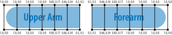
In Figure 9-5, the upper arm will be rigid on the left and curvy as it approaches the forearm. Conversely, the forearm will curve on the left and straighten out closer to the hand.
Let’s define some structures for the rendering engine, again leveraging the vector library in the appendix:
struct Vertex {  vec3 Position;
float Padding0;
vec2 TexCoord;
vec2 BoneWeights;
unsigned short BoneIndices;
unsigned short Padding1;
};
typedef std::vector<Vertex> VertexList;
typedef std::vector<GLushort> IndexList;
typedef std::vector<mat4> MatrixList;
struct Skeleton {
vec3 Position;
float Padding0;
vec2 TexCoord;
vec2 BoneWeights;
unsigned short BoneIndices;
unsigned short Padding1;
};
typedef std::vector<Vertex> VertexList;
typedef std::vector<GLushort> IndexList;
typedef std::vector<mat4> MatrixList;
struct Skeleton {  IndexList Indices;
VertexList Vertices;
};
struct SkinnedFigure {
IndexList Indices;
VertexList Vertices;
};
struct SkinnedFigure {  GLuint IndexBuffer;
GLuint VertexBuffer;
MatrixList Matrices;
};
GLuint IndexBuffer;
GLuint VertexBuffer;
MatrixList Matrices;
};
-
The
Vertexstructure is a POD type that defines the layout of the vertex buffer.-
The
Skeletonstructure encapsulates a relatively small set of points that make up an animated “stick figure.” We won’t be sending these points to OpenGL: it’s for internal purposes only, as you’ll see.-
The
SkinnedFigurestructure encapsulates the data that we’ll send to OpenGL. It contains handles for the static VBOs and a list of matrices that we’ll update at every frame.
Given a Skeleton object,
computing a list of model-view matrices is a bit tricky; see Example 9-6. This computes a sequence of matrices for the
joints along a single limb.
void ComputeMatrices(const Skeleton& skeleton, MatrixList& matrices)
{
    mat4 modelview = mat4::LookAt(Eye, Target, Up);

    float x = 0;
    IndexList::const_iterator lineIndex = skeleton.Indices.begin();
    for (int boneIndex = 0; boneIndex < BoneCount; ++boneIndex) {

        // Compute the length, orientation, and midpoint of this bone:
        float length;
        vec3 orientation, midpoint;
        {
            vec3 a = skeleton.Vertices[*lineIndex++].Position;
            vec3 b = skeleton.Vertices[*lineIndex++].Position;
            length = (b - a).Length();
            orientation = (b - a) / length;
            midpoint = (a + b) * 0.5f;
        }

        // Find the endpoints of the "unflexed" bone
        // that sits at the origin:
        vec3 a(0, 0, 0);
        vec3 b(length, 0, 0);
        if (StickFigureBones[boneIndex].IsBlended) {
            a.x += x;
            b.x += x;
        }
        x = b.x;

        // Compute the matrix that transforms the
        // unflexed bone to its current state:
        vec3 A = orientation;
        vec3 B = vec3(-A.y, A.x, 0);
        vec3 C = A.Cross(B);
        mat3 basis(A, B, C);
        vec3 T = (a + b) * 0.5;
        mat4 rotation = mat4::Translate(-T) * mat4(basis);
        mat4 translation = mat4::Translate(midpoint);
        matrices[boneIndex] = rotation * translation * modelview;
    }
}
}
}
-
Compute the primary model-view, which will be multiplied with each bone-specific transform.
-
Fill the columns of a change-of-basis matrix; to review the math behind this, flip back to Another Foray into Linear Algebra.
-
Translate the bone to the origin, and then rotate it around the origin.
-
-
Combine the primary model-view with the rotation and translation matrices to form the final bone matrix.
Skinning with OpenGL ES 2.0
Example 9-7 shows the vertex shader for skinning; this lies at the heart of the technique.
const int BoneCount = 17;

attribute vec4 Position;
attribute vec2 TextureCoordIn;
attribute vec2 BoneWeights;
attribute vec2 BoneIndices;

uniform mat4 Projection;
uniform mat4 Modelview[BoneCount];

varying vec2 TextureCoord;

void main(void)
{
    vec4 p0 = Modelview[int(BoneIndices.x)] * Position;
    vec4 p1 = Modelview[int(BoneIndices.y)] * Position;
    vec4 p = p0 * BoneWeights.x + p1 * BoneWeights.y;
    gl_Position = Projection * p;
    TextureCoord = TextureCoordIn;
}
Note that we’re applying only two bones at a time for this demo. By modifying the shader, you could potentially blend between three or more bones. This can be useful for situations that go beyond the classic elbow example, such as soft-body animation. Imagine a wibbly-wobbly blob that lurches around the screen; it could be rendered using a network of several “bones” that meet up at its center.
The fragment shader for the stick figure demo is incredibly simple; see Example 9-8. As you can see, all the real work for skinning is on the vertex shader side of things.
The ES 2.0 rendering code is fairly straightforward; see Example 9-9.
GLsizei stride = sizeof(Vertex);
mat4 projection = mat4::Ortho(-1, 1, -1.5, 1.5, -100, 100);

// Draw background:
...

// Render the stick figure:
glUseProgram(m_skinning.Program);

glUniformMatrix4fv(m_skinning.Uniforms.Projection, 1,
                   GL_FALSE, projection.Pointer());

glUniformMatrix4fv(m_skinning.Uniforms.Modelview,
                   m_skinnedFigure.Matrices.size(),
                   GL_FALSE,
                   m_skinnedFigure.Matrices[0].Pointer());

glBindTexture(GL_TEXTURE_2D, m_textures.Circle);
glEnable(GL_BLEND);
glBlendFunc(GL_SRC_ALPHA, GL_ONE_MINUS_SRC_ALPHA);

glEnableVertexAttribArray(m_skinning.Attributes.Position);
glEnableVertexAttribArray(m_skinning.Attributes.TexCoord);
glEnableVertexAttribArray(m_skinning.Attributes.BoneWeights);
glEnableVertexAttribArray(m_skinning.Attributes.BoneIndices);

glBindBuffer(GL_ELEMENT_ARRAY_BUFFER, m_skinnedFigure.IndexBuffer);
glBindBuffer(GL_ARRAY_BUFFER, m_skinnedFigure.VertexBuffer);

glVertexAttribPointer(m_skinning.Attributes.BoneWeights, 2,
                      GL_FLOAT, GL_FALSE, stride,
                      _offsetof(Vertex, BoneWeights));
glVertexAttribPointer(m_skinning.Attributes.BoneIndices, 2,
                      GL_UNSIGNED_BYTE, GL_FALSE, stride,
                      _offsetof(Vertex, BoneIndices));
glVertexAttribPointer(m_skinning.Attributes.Position, 3,
                      GL_FLOAT, GL_FALSE, stride,
                      _offsetof(Vertex, Position));
glVertexAttribPointer(m_skinning.Attributes.TexCoord, 2,
                      GL_FLOAT, GL_FALSE, stride,
                      _offsetof(Vertex, TexCoord));

size_t indicesPerBone = 12 + 6 * (NumDivisions + 1);
int indexCount = BoneCount * indicesPerBone;
glDrawElements(GL_TRIANGLES, indexCount, GL_UNSIGNED_SHORT, 0);
This is the largest number of attributes
we’ve ever enabled; as you can see, it can be quite a chore to set them
all up. One thing I find helpful is creating my own variant of the
offsetof macro, useful for passing a byte offset to
glVertexAttribPointer. Here’s how I define
it:
#define _offsetof(TYPE, MEMBER) (GLvoid*) (offsetof(TYPE, MEMBER))
The compiler will complain if you use
offsetof on a type that it doesn’t consider to be a
POD type. This is mostly done just to conform to the ISO C++ standard;
in practice, it’s usually safe to use offsetof on
simple non-POD types. You can turn off the warning by adding
-Wno-invalid-offsetof to the gcc command line. (To
add gcc command-line arguments in Xcode, right-click the source file,
and choose Get Info.)
Skinning with OpenGL ES 1.1
All Apple devices at the time of this writing
support the GL_OES_matrix_palette extension under
OpenGL ES 1.1. As you’ll soon see, it works in a manner quite similar to
the OpenGL ES 2.0 method previously discussed. The tricky part is that
it imposes limits on the number of so-called vertex units and palette
matrices.
Each vertex unit performs a single bone transformation. In the simple stick figure example, we need only two vertex units for each joint, so this isn’t much of a problem.
Palette matrices are simply another term for bone matrices. We need 17 matrices for our stick figure example, so a limitation might complicate matters.
Here’s how you can determine how many vertex units and palette matrices are supported:
int numUnits;
glGetIntegerv(GL_MAX_VERTEX_UNITS_OES, &numUnits);

int maxMatrices;
glGetIntegerv(GL_MAX_PALETTE_MATRICES_OES, &maxMatrices);
Table 9-1 shows the limits for current Apple devices at the time of this writing.
| Apple device | Vertex units | Palette matrices |
| First-generation iPhone and iPod touch | 3 | 9 |
| iPhone 3G and 3GS | 4 | 11 |
| iPhone Simulator | 4 | 11 |
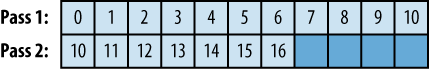
Uh oh, we need 17 matrices, but at most only
11 are supported! Fret not; we can simply split the rendering pass into
two draw calls. That’s not too shoddy! Moreover, since
glDrawElements allows us to pass in an offset, we can
still store the entire stick figure in only one VBO.
Let’s get down to the details. Since OpenGL ES 1.1 doesn’t have uniform variables, it supplies an alternate way of handing bone matrices over to the GPU. It works like this:
glEnable(GL_MATRIX_PALETTE_OES);
glMatrixMode(GL_MATRIX_PALETTE_OES);
for (int boneIndex = 0; boneIndex < boneCount; ++boneIndex) {
    glCurrentPaletteMatrixOES(boneIndex);
    glLoadMatrixf(modelviews[boneIndex].Pointer());
}
That was pretty straightforward! When you
enable GL_MATRIX_PALETTE_OES, you’re telling OpenGL
to ignore the standard model-view and instead use the model-views that
get specified while the matrix mode is set to
GL_MATRIX_PALETTE_OES.
We also need a way to give OpenGL the blend weights and bone indices. That is simple enough:
glEnableClientState(GL_WEIGHT_ARRAY_OES);
glEnableClientState(GL_MATRIX_INDEX_ARRAY_OES);

glMatrixIndexPointerOES(2, GL_UNSIGNED_BYTE, stride,
                        _offsetof(Vertex, BoneIndices));
glWeightPointerOES(2, GL_FLOAT, stride, _offsetof(Vertex, BoneWeights));
We’re now ready to write some rendering code, taking into account that the number of supported matrix palettes might be less than the number of bones in our model. Check out Example 9-10 to see how we “cycle” the available matrix slots; further explanation follows the listing.
const SkinnedFigure& figure = m_skinnedFigure;

// Set up for skinned rendering:
glMatrixMode(GL_MATRIX_PALETTE_OES);
glEnableClientState(GL_WEIGHT_ARRAY_OES);
glEnableClientState(GL_MATRIX_INDEX_ARRAY_OES);

glBindBuffer(GL_ELEMENT_ARRAY_BUFFER, figure.IndexBuffer);
glBindBuffer(GL_ARRAY_BUFFER, figure.VertexBuffer);

glMatrixIndexPointerOES(2, GL_UNSIGNED_BYTE, stride,
                        _offsetof(Vertex, BoneIndices));
glWeightPointerOES(2, GL_FLOAT, stride, _offsetof(Vertex, BoneWeights));
glVertexPointer(3, GL_FLOAT, stride, _offsetof(Vertex, Position));
glTexCoordPointer(2, GL_FLOAT, stride, _offsetof(Vertex, TexCoord));

// Make several rendering passes if need be,
// depending on the maximum bone count:
int startBoneIndex = 0;
while (startBoneIndex < BoneCount - 1) {

    int endBoneIndex = min(BoneCount, startBoneIndex + m_maxBoneCount);

    for (int boneIndex = startBoneIndex;
         boneIndex < endBoneIndex;
         ++boneIndex)
    {

        int slotIndex;

        // All passes beyond the first pass are offset by one.
        if (startBoneIndex > 0)
            slotIndex = (boneIndex + 1) % m_maxBoneCount;
        else
            slotIndex = boneIndex % m_maxBoneCount;

        glCurrentPaletteMatrixOES(slotIndex);
        mat4 modelview = figure.Matrices[boneIndex];
        glLoadMatrixf(modelview.Pointer());
    }

    size_t indicesPerBone = 12 + 6 * (NumDivisions + 1);
    int startIndex = startBoneIndex * indicesPerBone;
    int boneCount = endBoneIndex - startBoneIndex;

    const GLvoid* byteOffset = (const GLvoid*) (startIndex * 2);
    int indexCount = boneCount * indicesPerBone;
    glDrawElements(GL_TRIANGLES, indexCount,
                   GL_UNSIGNED_SHORT, byteOffset);

    startBoneIndex = endBoneIndex - 1;
}
Under our system, if the model has 17 bones and the hardware supports 11 bones, vertices affected by the 12th matrix should have an index of 1 rather than 11; see Figure 9-6 for a depiction of how this works.
Unfortunately, our system breaks down if at least one vertex needs to be affected by two bones that “span” the two passes, but this rarely occurs in practice.
Generating Weights and Indices
The limitation on available matrix palettes also needs to be taken into account when annotating the vertices with their respective matrix indices. Example 9-11 shows how our system generates the blend weights and indices for a single limb. This procedure can be used for both the ES 1.1-based method and the shader-based method; in this book’s sample code, I placed it in a base class that’s shared by both rendering engines.
for (int j = 0; j < NumSlices; ++j) {

    GLushort index0 = floor(blendWeight);
    GLushort index1 = ceil(blendWeight);
    index1 = index1 < BoneCount ? index1 : index0;

    int i0 = index0 % maxBoneCount;
    int i1 = index1 % maxBoneCount;

    // All passes beyond the first pass are offset by one.
    if (index0 >= maxBoneCount || index1 >= maxBoneCount) {
        i0++;
        i1++;
    }

    destVertex->BoneIndices = i1 | (i0 << 8);
    destVertex->BoneWeights.x = blendWeight - index0;
    destVertex->BoneWeights.y = 1.0f - destVertex->BoneWeights.x;
    destVertex++;

    destVertex->BoneIndices = i1 | (i0 << 8);
    destVertex->BoneWeights.x = blendWeight - index0;
    destVertex->BoneWeights.y = 1.0f - destVertex->BoneWeights.x;
    destVertex++;

    blendWeight += (j < NumSlices / 2) ? delta0 : delta1;
}
In Example 9-11, the
delta0 and delta1 variables are
the increments used for each half of limb; refer to Table 9-2 and flip back to Figure 9-5 to see how this works.
| Limb | Increment |
| First half of upper arm | 0 |
| Second half of upper arm | 0.166 |
| First half of forearm | 0.166 |
| Second half of forearm | 0 |
For simplicity, we’re using a linear falloff of bone weights here, but I encourage you to try other variations. Bone weight distribution is a bit of a black art.
That’s it for the skinning demo! As always, you can find the complete sample code on this book’s website. You might also want to check out the 3D skinning demo included in the PowerVR SDK.
Watch Out for Pinching
Before you get too excited, I should warn you that vertex skinning isn’t a magic elixir. An issue called pinching has caused many a late night for animators and developers. Pinching is a side effect of interpolation that causes severely angled joints to become distorted (Figure 9-7).

If you’re using OpenGL ES 2.0 and pinching is causing headaches, you should research a technique called dual quaternion skinning, developed by Ladislav Kavan and others.
Further Reading
The list of optimizations in this chapter is by no means complete. Apple’s “OpenGL ES Programming Guide” document, available from the iPhone developer site, has an excellent list of up-to-date advice. Imagination Technologies publishes a similar document that’s worth a look.
Since we’re at the end of this book, I’d also like to point out a couple resources for adding to your general OpenGL skills. OpenGL Shading Language (Addison-Wesley Professional) by Randi Rost provides a tight focus on shader development. Although this book was written for desktop GLSL, the shading language for ES is so similar to standard GLSL that almost everything in Randi’s book can be applied to OpenGL ES as well.
The official specification documents for OpenGL ES are available as PDFs at the Khronos website:
| http://www.khronos.org/registry/gles/ |
The OpenGL specs are incredibly detailed and unambiguous. I find them to be a handy reference, but they’re not exactly ideal for casual armchair reading. For a more web-friendly reference, check out the HTML man pages at Khronos:
| http://www.khronos.org/opengles/sdk/docs/man/ |
In the end, one of the best ways to learn is to play—write some 3D iPhone apps from the ground up, and enjoy yourself!
Get iPhone 3D Programming now with the O’Reilly learning platform.
O’Reilly members experience books, live events, courses curated by job role, and more from O’Reilly and nearly 200 top publishers.

