Investment Theory and Risk Management, + Website

Appendix 10.1: Active Space

For active portfolios consisting of many benchmarks, it is often convenient to compress the various benchmarks into a single composite benchmark. That way, we compare k active portfolios to a single benchmark. It not only reduces the dimensionality of the problem from 2k × 2k to a (k + 1) × (k + 1) problem, but simplifies computations and interpretations of active risk. What we need to do, therefore, is to somehow aggregate the benchmarks into a single overall benchmark and compare all the active holdings to this single benchmark. Admittedly, that is not intuitive, but we can hope that it will make more sense after I develop the concept for you.

First, I construct a special matrix that will aggregate the benchmark variances and covariances into a single row and column. For the two-asset case it looks like this:

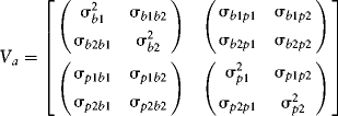
Recall V_a:

Aggregating the benchmarks is accomplished by m′V_am, which reduces to:

Thus, where we started with a 2k × 2k active covariance matrix, we now work with a matrix of dimension k + 1, in which the first row and column summarize the covariances between the benchmarks and portfolios (or assets). The 2 × 2 diagonal submatrix in the lower right ...