Pitfalls of Trend Analysis
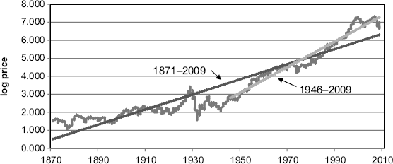
Anchoring on linear time trends as a basis to support returns forecasts also appeal to mean reversion logic. This is illustrated in Figure 4.2.
Figure 4.2 S&P 500 Trend Growth

Superimposed on the (log) price history of the index are two trend lines—trend growth from January 1871 to December 2009, which is 4.27 percent annual growth and annual trend growth after World War II (January 1946 to December 2009) at 7.35 percent. These are monthly index values. Trend growth is estimated by regressing ln(Price) = α + β time and computing annual growth in percent using 100∗((1 + β)12 – 1). These are clearly distinct trend estimates, and the conclusions drawn from mean reversion arguments are naturally going to be sensitive to which trend one is referring to. To see how sensitive trend estimates are, consider that the annual trend growth in the S&P was 1.88 percent from 1871 to 1928, 5.86 percent from 1929 to 1989, 6.81 percent from 1929 to 2009 and, as mentioned before, 7.35 percent from 1946 to 2009. This is a rather wide range and, depending on which trend line we use, mean reversion from any given spot index level may be up or down!
For example, historically, when the level of the S&P 500 was as far below the post–World War II trend as it was on, say, April 30, 2009, the subsequent average 10-year return was 13.44 percent. Many market analysts pointed to this ...
Get Investment Theory and Risk Management, + Website now with the O’Reilly learning platform.
O’Reilly members experience books, live events, courses curated by job role, and more from O’Reilly and nearly 200 top publishers.

