8The Finite Difference Method
8.1 Introduction and a Simple Example
We begin this chapter by examining a two-dimensional (2d) rectangular structure. Extending the analysis to three-dimensional (3d) structures in rectangular, cylindrical, or spherical coordinates is straightforward and will be discussed later. Also, for now consider only prescribed voltage boundary conditions.
Laplace’s equation in rectangular coordinates is
For a uniform structure infinitely long in the Z direction, all partial derivatives with respect to Z vanish, leaving us with the 2d equation
Figure 8.1 shows a rectangular grid of points in 2d space.
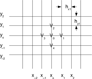
FIGURE 8.1 A rectangular grid of points.
The lines in the figure are just for our eyes to follow easily. Of interest are the intersections of these lines, which we’ll call nodes. The X-axis separation of nodes is hx [equation (8.3)]; the Y-axis separation of nodes is hy [equation (8.4)]:
For now, assume that hx = hy = h.
Voltages at the nodes are ...
Get Introduction to Numerical Electrostatics Using MATLAB now with the O’Reilly learning platform.
O’Reilly members experience books, live events, courses curated by job role, and more from O’Reilly and nearly 200 top publishers.

