Chapter 1. What Is a Model?
There was a time in my undergraduate physics studies that I was excited to learn what a model was. I remember the scene pretty well. We were in a Stars and Galaxies class, getting ready to learn about atmospheric models that could be applied not only to the Earth, but to other planets in the solar system as well. I knew enough about climate models to know they were complicated, so I braced myself for an onslaught of math that would take me weeks to parse. When we finally got to the meat of the subject, I was kind of let down: I had already dealt with data models in the past and hadn’t even realized!
Because models are a fundamental aspect of machine learning, perhaps it’s not surprising that this story mirrors how I learned to understand the field of machine learning. During my graduate studies, I was on the fence about going into the financial industry. I had heard that machine learning was being used extensively in that world, and, as a lowly physics major, I felt like I would need to be more of a computational engineer to compete. I came to a similar realization that not only was machine learning not as scary of a subject as I originally thought, but I had indeed been using it before. Since before high school, even!
Models are helpful because unlike dashboards, which offer a static picture of what the data shows currently (or at a particular slice in time), models can go further and help you understand the future. For example, someone who is working on a sales team might only be familiar with reports that show a static picture. Maybe their screen is always up to date with what the daily sales are. There have been countless dashboards that I’ve seen and built that simply say “this is how many assets are in right now.” Or, “this is what our key performance indicator is for today.” A report is a static entity that doesn’t offer an intuition as to how it evolves over time.
Figure 1-1 shows what a report might look like:
op<-par(mar=c(10,4,4,2)+0.1)#margin formattingbarplot(mtcars$mpg,names.arg=row.names(mtcars),las=2,ylab="FuelEfficiency in Miles per Gallon")
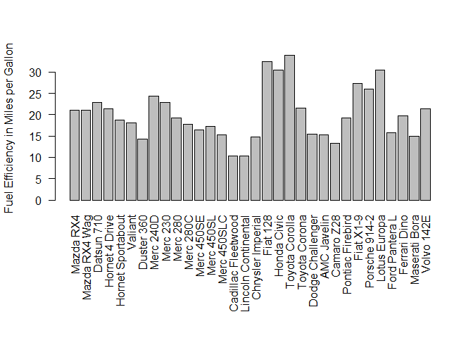
Figure 1-1. A distribution of vehicle fuel efficiency based on the built-in mtcars dataset found in R
Figure 1-1 depicts a plot of the mtcars dataset that comes prebuilt with R.
The figure shows a number of cars plotted by their fuel efficiency in miles
per gallon. This report isn’t very interesting. It
doesn’t give us any predictive power. Seeing how the efficiency of the
cars is distributed is nice, but how can we relate that to other things
in the data and, moreover, make predictions from it?
A model is any sort of function that has predictive power.
So how do we turn this boring report into something more useful? How do we bridge the gap between reporting and machine learning? Oftentimes the correct answer to this is “more data!” That can come in the form of more observations of the same data or by collecting new types of data that we can then use for comparison.
Let’s take a look at the built-in mtcars dataset that comes with R in
more detail:
head(mtcars)
##                    mpg cyl disp  hp drat    wt  qsec vs am gear carb
## Mazda RX4         21.0   6  160 110 3.90 2.620 16.46  0  1    4    4
## Mazda RX4 Wag     21.0   6  160 110 3.90 2.875 17.02  0  1    4    4
## Datsun 710        22.8   4  108  93 3.85 2.320 18.61  1  1    4    1
## Hornet 4 Drive    21.4   6  258 110 3.08 3.215 19.44  1  0    3    1
## Hornet Sportabout 18.7   8  360 175 3.15 3.440 17.02  0  0    3    2
## Valiant           18.1   6  225 105 2.76 3.460 20.22  1  0    3    1
By just calling the built-in object of mtcars within R, we can see all
sorts of columns in the data from which to choose to build a
machine learning model. In the machine learning world, columns of data
are sometimes also called features. Now that we know what we have to work
with, we could try seeing if there’s a relationship between the car’s
fuel efficiency and any one of these features, as depicted in Figure 1-2:
pairs(mtcars[1:7],lower.panel=NULL)
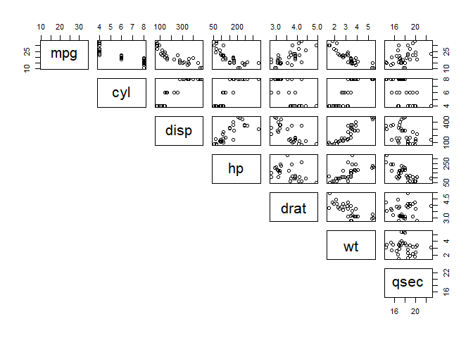
Figure 1-2. A pairs plot of the mtcars dataset, focusing on the first seven rows
Each box is its own separate plot, for which the dependent variable is the text box at the bottom of the column, and the independent variable is the text box at the beginning of the row. Some of these plots are more interesting for trending purposes than others. None of the plots in the cyl row, for example, look like they lend themselves easily to simple regression modeling.
In this example, we are plotting some of those features against others. The columns, or features, of this data are defined as follows:
- mpg
-
Miles per US gallon
- cyl
-
Number of cylinders in the car’s engine
- disp
-
The engine’s displacement (or volume) in cubic inches
- hp
-
The engine’s horsepower
- drat
-
The vehicle’s rear axle ratio
- wt
-
The vehicle’s weight in thousands of pounds
- qsec
-
The vehicle’s quarter-mile race time
- vs
-
The vehicle’s engine cylinder configuration, where “V” is for a v-shaped engine and “S” is for a straight, inline design
- am
-
The transmission of the vehicle, where 0 is an automatic transmission and 1 is a manual transmission
- gear
-
The number of gears in the vehicle’s transmission
- carb
-
The number of carburetors used by the vehicle’s engine
You can read the upper-right plot as “mpg as a function of quarter-mile-time,” for example. Here we are mostly interested in something that looks like it might have some kind of quantifiable relationship. This is up to the investigator to pick out what patterns look interesting. Note that “mpg as a function of cyl” looks very different from “mpg as a function of wt.” In this case, we focus on the latter, as shown in Figure 1-3:
plot(y=mtcars$mpg,x=mtcars$wt,xlab="Vehicle Weight",ylab="Vehicle Fuel Efficiency in Miles per Gallon")
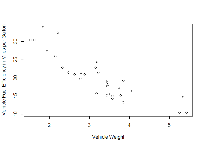
Figure 1-3. This plot is the basis for drawing a regression line through the data
Now we have a more interesting kind of dataset. We still have our fuel efficiency, but now it is plotted against the weight of the respective cars in tons. From this kind of format of the data, we can extract a best fit to all the data points and turn this plot into an equation. We’ll cover this in more detail in later chapters, but we use a function in R to model the value we’re interested in, called a response, against other features in our dataset:
mt.model<-lm(formula=mpg~wt,data=mtcars)coef(mt.model)[2]
##        wt
## -5.344472
coef(mt.model)[1]
## (Intercept)
##    37.28513
In this code chunk, we modeled the vehicle’s fuel efficiency (mpg) as a function of the vehicle’s weight (wt) and extracted values from that model object to use in an equation that we can write as follows:
- Fuel Efficiency = 5.344 × Vehicle Weight + 37.285
Now if we wanted to know what the fuel efficiency was for any car, not just those in the dataset, all we would need to input is the weight of it, and we get a result. This the benefit of a model. We have predictive power, given some kind of input (e.g., weight), that can give us a value for any number we put in.
The model might have its limitations, but this is one way in which we can help to expand the data beyond a static report into something more flexible and more insightful. A given vehicle’s weight might not actually be predictive of the fuel efficiency as given by the preceding equation. There might be some error in the data or the observation.
You might have come across this kind of modeling procedure before in dealing with the world of data. If you have, congratulations—you have been doing machine learning without even knowing it! This particular type of machine learning model is called linear regression. It’s much simpler than some other machine learning models like neural networks, but the algorithms that make it work are certainly using machine learning principles.
Algorithms Versus Models: What’s the Difference?
Machine learning and algorithms can hardly be separated. Algorithms are another subject that can seem impenetrably daunting at first, but they are actually quite simple at their core, and you have probably been using them for a long time without realizing it.
An algorithm is a set of steps performed in order.
That’s all an algorithm is. The algorithm for putting on your shoes might be something like putting your toes in the open part of the shoe, and then pressing your foot forward and your heel downward. The set of steps necessary to produce a machine learning algorithm are more complicated than designing an algorithm for putting on your shoes, of course, but one of the goals of this book is to explain the inner workings of the most widely used machine learning models in R by helping to simplify their algorithmic processes.
The simplest algorithm for linear regression involves putting two points on a plot and then drawing a line between them. You get the important parts of the equation (slope and intercept) by taking the difference in the coordinates of those points with respect to some origin. The algorithm becomes more complicated when you try to do the same procedure for more than two points, however. That process involves more equations that can be tedious to compute by hand for a human but very easy for a processor in a computer to handle in microseconds.
A machine learning model like regression or clustering or neural networks relies on the workings of algorithms to help them run in the first place. Algorithms are the engine that underlie the simple R code that we run. They do all the heavy lifting of multiplying matrices, optimizing results, and outputting a number for us to use. There are many types of models in R, which span an entire ecosystem of machine learning more generally. There are three major types of models: regression models, classification models, and mixed models that are a combination of both. We’ve already encountered a regression model. A classification model is different in that we would be trying to take input data and arrange it according to a type, class, group, or other discrete output. Mixed models might start with a regression model and then use the output from that to help it classify other types of data. The reverse could be true for other mixed models.
The function call for a simple linear regression in R can be written as:
lm(y ~ x), or read out loud as “give me the linear model for the
variable y as a function of the feature x.” What you’re not seeing
are the algorithms that the code is running to make optimizations based
on the data that we give it.
In many cases, the details of these algorithms are beyond the scope of this book, but you can look them up easily. It’s very easy to become lost in the weeds of algorithms and statistics when you’re simply trying to understand what the difference between a logistic regression machine learning model is compared to a support vector machine model.
Although documentation in R can vary greatly in quality from one machine learning function to the next, in general, one can look up the inner workings of a model by pulling up the help file for it:
?(lm)
From this help file, you can get a wealth of information on how the function itself works with inputs and what it outputs. Moreover, if you want to know the specific algorithms used in its computation, you might find it here or under the citations listed in the “Author(s)” or “References” sections. Some models might require an extensive digging process to get the exact documentation you are looking for, however.
A Note on Terminology
The word “model” is rather nebulous and difficult to separate from something
like a “function” or an “equation.” At the beginning of the chapter, we made a report. That was a static object that didn’t have any
predictive power. We then delved into the data to find another variable
that we could use as a modeling input. We used the lm() function
which gave us an equation at the end. We can quickly define these terms
as follows:
- Report
- Function
-
An object that has some kind of processing power, likely sits inside a model.
- Model
-
A complex object that takes an input parameter and gives an output.
- Equation
-
A mathematical representation of a function. Sometimes a mathematical model.
- Algorithm
-
A set of steps that are passed into a model for calculation or processing.
There are cases in which we use functions that might not yield mathematical results. For example, if we have a lot of data but it’s in the wrong form, we might develop a process by which we reshape the data into something more usable. If we were to model that process, we could have something more like a flowchart instead of an equation for us to use.
Many times these terms can be used interchangeably, which can be
confusing. In some respects, specific terminology is not that important,
but knowing that algorithms build into a model is important. The lm()
code is itself a function, but it’s also a linear model. It calls a
series of algorithms to find the best values that are then output as a
slope and an intercept. We then use those slopes and intercepts to build
an equation, which we can use for further analysis.
Modeling Limitations
Statistician George Box is often quoted for the caveat, “All models are wrong, but some are useful.” A model is a simplified picture of reality. In reality, systems are complex and ever changing. The human brain is phenomenal at being able to discover patterns and make sense of the universe around us, but even our senses are limited. All models, be they mathematical, computational, or otherwise are limited by the same human brain that designs them.
Here’s one classic example of the limits of a model: in the 1700s, Isaac Newton had developed a mathematical formulation describing the motions of objects. It had been well tested and was taken, more or less, to be axiomatic truth. Newton’s universal law of gravitation had been used with great success to describe how the planets move around the Sun. However, one outlier wasn’t well understood: the orbit of Mercury. As the planet Mercury orbits the Sun, its perihelion (the closest point to the Sun of its orbit) moves around ever so slightly over time. For the longest time, physicists couldn’t account for the discrepancy until the early twentieth century when Albert Einstein reformulated the model with his General Theory of Relativity.
Even Einstein’s equations break down at a certain level, however. Indeed, when new paradigms are discovered in the world of science, be they from nature throwing us a curve ball or when we discover anomalous data in the business world, models need to be redesigned, reevaluated, or reimplemented to fit the observations.
Coming back to our mtcars example, the limitations of our model come
from the data, specifically the time they were collected and the number
of data points. We are making rather bold assumptions about the fuel
efficiencies of cars today if we try to input just the weight of a
modern vehicle into a model that was built entirely from cars
manufactured in the 1970s. Likewise, there are very few data points in
the set to begin with. Thirty-two data points is pretty low to be making
be-all-end-all statements about any car’s fuel efficiency.
The limitations we have to caveat our mtcars model with are therefore
bound in time and in observations. We could say, “This is a model for
fuel efficiency of cars in the 1970s based on 32 different makes and
models.” We could not say, “This is a model for any car’s fuel
efficiency.”
Different models have different specific limitations as well. We will
dive into more statistical detail later, but developing something like a
simple linear regression model will come with some kind of error with it.
The way we measure that error is very different compared to how we
measure the error for a model like a kmeans clustering model, for
example. It’s important to be cognizant of error in a model to begin
with, but also how we compare errors between models of different
types.
When George Box says all models are wrong, he means that all models have some kind of error attributed to them. Regression models have a specific way of measuring error called the coefficient of determination, often referred to as the “R-squared” value. This is a measure of how close the data fits the model fitted line with values ranging from 0 to 1. A regression model with an R2 = 0.99 is quite a good linear fit to the data it’s modeling, but it’s not a 100% perfect mapping. Box goes on to say:1
Now it would be very remarkable if any system existing in the real world could be exactly represented by any simple model. However, cunningly chosen parsimonious models often do provide remarkably useful approximations. For example, the law PV = RT relating pressure P, volume V, and temperature T of an “ideal” gas via a constant R is not exactly true for any real gas, but it frequently provides a useful approximation and furthermore its structure is informative since it springs from a physical view of the behavior of gas molecules. For such a model there is no need to ask the question “Is the model true?” If “truth” is to be the “whole truth,” the answer must be “No.” The only question of interest is, “Is the model illuminating and useful?”
Without getting too deep into the weeds of the philosophy of science, machine learning modeling in all its forms is just an approximation of the universe that we are studying. The power in a model comes from its usefulness, which can stem from how accurate it can make predictions, nothing more. A model might be limited by its computational speed or its ability to be simply explained or utilized in a particular framework, as well. It’s important, therefore, to experiment and test data with many types of models and for us to choose what fits best with what our goals are. Implementing a regression model on a computational backend of a server might be far simpler to implement than a random forest regression model, for which there might be a trade-off in accuracy of a small amount.
Statistics and Computation in Modeling
When we think of machine learning, in a naive sense we think almost
exclusively about computers. As we shall see throughout the book,
machine learning has its basis in mathematics and statistics. In fact,
you could do all machine learning calculations by hand by using
only math. However, such a process becomes unsustainable depending on
the algorithm after only a few data points. Even the simple linear
regression model we worked on earlier this chapter becomes exponentially
more complicated when we move from two to three data points. However, modern
programming languages have so many built-in functions and packages that
it’s almost impossible to not have a regression function that takes one
line of code to get the same result in a fraction of the time. You have
seen this application thus far with the lm() function call in R
already. Most of the time, a robust statistical understanding is
paramount to understanding the inner workings of a machine learning
algorithm. Doubly so if you are asked by a colleague to explain why you
used such an algorithm.
In this book, we explore the mathematics behind the workings of these algorithms to an extent that it doesn’t overwhelm the focus on the R code and best practices therein. It can be quite eye opening to understand how a regression model finds the coefficients that we use to build the equation, especially given that some of the algorithms used to compute the coefficients can show up in other machine learning models and functions wholly different from linear regression.
With linear regression as our example, we might be interested in the statistics that define the model accuracy. There are numerous to list, and some that are too statistical for an introductory text, but a general list would include the following:
- Coefficient of determination
-
Sometimes listed as R2, this is how well the data fits to the modeled line for regression analyses.
- p-values
-
These are measures of statistical validity, where if your p-value is below 0.05, the value you are examining is likely to be statistically valid.
- Confidence intervals
-
These are two values between which we expect a parameter to be. For example, a 95% confidence interval between the numbers 1 and 3 might describe where the number 2 sits.
We can use these to understand the difference between a model that fits the data well and one that fits poorly. We can assess which features are useful for us to use in our model and we can determine the accuracy of the answers produced by the model.
The basic mathematical formulation of regression modeling with two data points is something often taught at the middle school level, but rarely does the theory move beyond that to three or more data points. The reason being that to calculate coefficients that way, we need to employ some optimization techniques like gradient descent. These are often beyond the scope of middle school mathematics but are an important underpinning of many different models and how they get the most accurate numbers for us to use.
We elaborate on concepts like gradient descent in further detail, but we leave that for the realm of the appendixes. It’s possible to run machine learning models without knowing the intricate details of the optimizations behind them, but when you get into more advanced model tuning, or need to hunt for bugs or assess model limitations, it’s essential to fully grasp the underpinnings of the tools you are working with.
Data Training
One statistical method that we cover in detail is that of training data. Machine learning requires us to first train a data model, but what does that mean exactly? Let’s say that we have a model for which we have some input that goes through an algorithm that generates an output. We have data for which we want a prediction, so we pass it through the model and get a result out. We then evaluate the results and see if the associated errors in the model go down or not. If they do, we are tuning the model in the right direction, otherwise if the errors continue to build up, we need to tweak our model further.
It’s very important for us to not train our machine learning models on data that we then pass back into it in order to test its validity. If, for example, we train a black box model on 50 data points and then pass those same 50 data points back through the model, the result we get will be suspiciously accurate. This is because our black box example has already seen the data so it basically knows the right answer already.
Often our hands are tied with data availability. We can’t pass data we don’t have into a model to test it and see how accurate it is. If, however, we took our 50-point dataset and split it in such a way that we used a majority of the data points for training but leave some out for testing, we can solve our problem in a more statistically valid way. The danger with this is splitting into training and test sets when we have only a small number of data points to begin with. But if we were limited in observations to start, using advanced machine learning techniques might not be the best approach anyway.
Now if we have our 50-point dataset and split it so that 80% of our data went into the training set (40 data points) and the rest went into our test set, we can better assess the model’s performance. The black box model will be trained on data that’s basically the same form as the test set (hopefully), but the black box model hasn’t seen the exact data points in the test set yet. After the model is tuned and we give it the test set, the model can make some predictions without the problem of being biased as a result of data it has seen before.
Methods of splitting up data for training and testing purposes are known as sampling techniques. These can come in many flavors like taking the top 40 rows of data as the training set, taking random rows from our data, or more advanced techniques.
Cross-Validation
Training data is very valuable to tuning machine learning models. Tuning a machine learning model is when you have a bunch of inputs whose values we can change slightly without changing the underlying data. For example, you might have a model that has three parameters that you can tune as follows: A=1, B=2, C=“FALSE”. If your model doesn’t turn out right, you can tweak it by changing the values to A=1.5, B=2.5, C=“FALSE”, and so forth with various permutations.
Many models have built-in ways to ingest data, perform some operations on it, and then save the tuned operations to a data structure that is used on the test data. In many cases during the training phase, you might want to try other statistical techniques like cross-validation. This is sort of like another mini-step of splitting into training and test sets and running the model, but only on the training data. For example, you take your 50-point total dataset and split 80% into a training set, leaving the rest for your final test phase. We are left with 40 rows with which to train your data model. You can split these 40 rows further into a 32-row training set and an 8-row test set. By doing so and going through a similar training and test procedure, you can get an ensemble of errors out of your model and use those to help refine its tuning even further.
Some examples of cross-validation techniques in R include the following:
-
Bootstrap cross-validation
-
Bootstrap 632 cross-validation
-
k-fold cross-validation
-
Repeated cross-validation
-
Leave-one-out cross-validation
-
Leave-group-out cross-validation
-
Out-of-bag cross-validation
-
Adaptive cross-validation
-
Adaptive bootstrap cross-validation
-
Adaptive leave-group-out cross-validation
We expand on these methods later; their usage is highly dependent on the structure of the data itself. The typical gold standard of cross-validation techniques is k-fold cross-validation, wherein you pick k = 10 folds against which to validate. This is the best balance between efficient data usage and avoiding splits in the data that might be poor choices. Chapter 3 looks at k-fold cross-validation in more detail.
Why Use R?
In this book, we provide a gentle introduction to the world of machine learning as illustrated with code and examples from R. The R language is a free, open source programming language that has its legacy in the world of statistics, being primarily built off of S and subsequently S+. So even though the R language itself has not been around for too long, there is some historical legacy code from its predecessors that have a good syntactic similarity to what we see today. The question is this: why use R in the first place? There are so many programming languages to choose from, how do you know which one is the best for what you want to accomplish?
The Good
R has been growing in popularity at an explosive rate. Complementary
tools to learn R have also grown, and there are no shortage of great
web-based tutorials and courses to choose from. One package, swirl,
can even teach you how to use R from within the console itself. Many
online courses also do instruction through swirl as well.
Some cover simple data analysis, others cover more complex topics like
mathematical biostatistics.
R also has great tools for accessibility and reproduction of work. Web
visualizations like the package shiny make it possible for you to build interactive
web applications that can be used by non-experts to interact with
complex datasets without the need to know or even install R.
There are a number of supported integrated development environments (IDEs) for R, but the most popular one is R Studio, as shown in Figure 1-4.
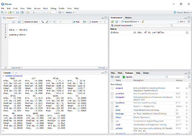
Figure 1-4. R Studio is a free integrated development environment (IDE) for R that is very stable and user-friendly for those new to the language
In fact, this book is being written in R Studio, using R Markdown. R supports a version of Markdown, a lightweight language that you can convert to all sorts of forms for display on the web or rendered to PDF files. It’s a great way to share code via publishing on the web or to write professional documentation. Doing so gives you the ability to write large swaths of text but also provide graphical examples such as those shown earlier in the chapter.
Another powerful feature of the language is support for data frames. Data frames are like a SQL database in memory that allow you to reshape and manipulate data to summarize and carry out lots of valuable data processing. Unlike a traditional matrix of data in which every column is the same data type, data frames allow you to mix them up. There will be countless times as you work with data when you will have a “Name” field with character data in it, followed by some numerical columns like “ID” or “Sales.” Reading that data into some languages can cause a problem if you can’t mix and match the data types of the columns.
In the next example, we have three vectors of different types: one numeric, one a vector of factors, and one a vector of logical values. Using data frames, you can combine all of these into a single dataset. More often than not, in the data science world we work with data of mixed types in the same table. Oftentimes, that can be helpful for subsetting the table based on certain criteria for analytical work.
v1=c(1,2,3)v2=c("Jerry","George","Elaine")v3=c(TRUE,FALSE,TRUE)data_frame=data.frame(v1,v2,v3)str(data_frame)
## 'data.frame': 3 obs. of 3 variables:## $ v1: num 1 2 3## $ v2: Factor w/ 3 levels "Elaine","George",..: 3 2 1## $ v3: logi TRUE FALSE TRUE
Data manipulation takes a majority of the time for those involved in
data analysis, and R has several packages to facilitate that work. The
dplyr package is a fantastic way to reshape and manipulate data in a
verbiage that makes intuitive sense. The lubridate package is a
powerful way to do manipulation on tricky datetime-formatted data.
With the dplyr package comes the pipe operator, %>%. This helpful
tool allows you to simplify code redundancy. Instead of assigning a
variable var1 an input and then using that input in another stage named
var2, and so on, you can use this pipe operator as a “then do” part of
your code.
R and Machine Learning
R has a lot of good machine learning packages. Some of which you can see on the CRAN home page. Yet the list of actual machine learning models is much greater. There are more than 200 types of machine learning models that are reasonably popular in the R ecosystem, and there are fairly strict rules governing each one.
The appendix includes a comprehensive list of more than 200 functions; their package dependencies, if they are used for classification, regression, or both; and any keywords used with them.
We have selected R for this book because machine learning has its basis in statistics, and R is well suited to illustrate those relationships. The ecosystem of statistical modeling packages in R is robust and user-friendly for the most part. Managing data in R is a big part of a data scientist’s day-to-day functionality, and R is very well developed for such a task. Although R is robust and relatively easy to learn from a data science perspective, the truth is that there is no single best programming language that will cover all your needs. If you are working on a project that requires the data to be in some specific form, there might be a language that has a package already built for that structure of data to a great degree of accuracy and speed. Other times, you might need to build your own solution from scratch.
R offers a fantastic tool for helping with the modeling process, known
as the function operator, ~. This symbolic operator acts like an
equals sign in a mathematical formula. Earlier we saw the example with a
linear model in which we had lm(mtcars$mpg ~ mtcars$wt). In that case,
mtcars$mpg was our response, the item we want to model as the output,
and mtcars$wt was the input. Mathematically, this would be like
y = f(x) in mathematical notation compared with y ~ x in R code.
This powerful operator makes it possible for you to utilize multiple inputs very easily. We might expect to encounter a multivariate function in mathematics to be written as follows:
- y = f(x1, x2, x3, ...)
In R, that formulation is very straightforward:
y~x_1+x_2+x_3
What we are doing here is saying that our modeling output y is not only a
function of x_1, but many other variables, as well. We will see in
dedicated views of machine learning models how we can utilize multiple
features or inputs in our models.
The Bad
R has some drawbacks, as well. Many algorithms in its ecosystem are provided by the community or other third parties, so there can be some inconsistency between them and other tools. Each package in R is like its own mini-ecosystem that requires a little bit of understanding first before going all out with it. Some of these packages were developed a long time ago and it’s not obvious what the current “killer app” is for a particular machine learning model. You might want to do a simple neural network model, for example, but you also want to visualize it. Sometimes, you might need to select a package you’re less familiar with for its specific functionality and leave your favorite one behind.
Sometimes, documentation for more obscure packages can be inconsistent, as
well. As referenced earlier, you can pull up the help file or manual
page for a given function in R by doing something like ?lm() or
?rf(). In a lot of cases, these include helpful examples at the bottom
of the page for how to run the function. However, some cases are
needlessly complex and can be simplified to a great extent. One goal of
this book is to try to present examples in the simplest cases to build
an understanding of the model and then expand on the complexity of its
workings from there.
Finally, the way R operates from a programmatic standpoint can drive some professional developers up a wall with how it handles things like type casting of data structures. People accustomed to working in a very strict object-oriented language for which you allocate specific amounts of memory for things will find R to be rather lax in its treatment of boundaries like those. It’s easy to pick up some bad habits as a result of such pitfalls, but this book aims to steer clear of those in favor of simplicity to explain the machine learning landscape.
Summary
In this chapter we’ve scoped out the vision for our exploration of machine learning using the R programming language.
First we explored what makes up a model and how that differs from a
report. You saw that a static report doesn’t tell us much in terms of
predictability. You can turn a report into something more like a model by
first introducing another feature and examining if there is some kind of
relationship in the data. You then fit a simple linear regression model
using the lm() function and got an equation as your final result. One
feature of R that is quite powerful for developing models is the
function operator ~. You can use this function with great effect for
symbolically representing the formulas that you are trying to model.
We then explored the semantics of what defines a model. A machine
learning model like linear regression utilizes algorithms like gradient
descent to do its background optimization procedures. You call linear
regression in R by using the lm() function and then extract the coefficients
from the model, using those to build your equation.
An important step with machine learning and modeling in general is to
understand the limits of the models. Having a robust model of a complex
set of data does not prevent the model itself from being limited in
scope from a time perspective, like we saw with our mtcars data.
Further, all models have some kind of error tied to them. We
explore error assessment on a model-by-model basis, given that we can’t directly
compare some types to others.
Lots of machine learning models utilize complicated statistical algorithms for them to compute what we want. In this book, we cover the basics of these algorithms, but focus more on implementation and interpretation of the code. When statistical concepts become more of a focus than the underlying code for a given chapter, we give special attention to those concepts in the appendixes where appropriate. The statistical techniques that go into how we shape the data for training and testing purposes, however, are discussed in detail. Oftentimes, it is very important to know how to specifically tune the machine learning model of choice, which requires good knowledge of how to handle training sets before passing test data through the fully optimized model.
To cap off this chapter, we make the case for why R is a suitable tool for machine learning. R has its pedigree and history in the field of statistics, which makes it a good platform on which to build modeling frameworks that utilize those statistics. Although some operations in R can be a little different than other programming languages, on the whole R is a relatively simple-to-use interface for a lot of complicated machine learning concepts and functions.
Being an open source programming language, R offers a lot of cutting-edge machine learning models and statistical algorithms. This can be a double-edged sword in terms of help files or manual pages, but this book aims to help simplify some of the more impenetrable examples encountered when looking for help.
In Chapter 2, we explore some of the most popular machine learning models and how we use them in R. Each model is presented in an introductory fashion with some worked examples. We further expand on each subject in a more in-depth dedicated chapter for each topic.
1 Box, G. E. P., J. S. Hunter, and W. G. Hunter. Statistics for Experimenters. 2nd ed. John Wiley & Sons, 2005.
Get Introduction to Machine Learning with R now with the O’Reilly learning platform.
O’Reilly members experience books, live events, courses curated by job role, and more from O’Reilly and nearly 200 top publishers.

