Chapter 4. All the Roads to Nowhere: How keeping things in balance is the essence of control.
“Plus ça change, plus c’est la měme chose.”
(The more everything changes, the more it all stays the same)
Jean-Baptiste Alphonse Karr
Don’t move! Stay where you are! Don’t leave town! Don’t go anywhere!
Let’s hope these are not phrases you have had occasion to hear very often, at least outside of fiction. They are arresting exclamations, challenging someone to stay put, i.e. maintain a stable location, with varying degrees of accuracy—which is a turgid way of saying that they describe a status quo. One could also say that they are different ways of expressing an absence of change, at different scales: they represent different approximations to staying put. The sequence starts with millimetre movements of your muscles, then relaxes to your immediate surroundings, falls back to a geographic region, and finally gives up altogether being specific about location.
We understand these vague concepts intuitively. Our brains’ semantic analyzers regularly decode such patterns of words, and attach meaning to them in the context of a scenario. That is the power of the human mind. If someone says, “I didn’t move for 20 years”, this does not mean that they were frozen in liquid nitrogen for two decades. It probably means that they settled in the same home, in the same town, i.e. that their average position remained within some general threshold radius, even allowing for one or two excursions to holiday destinations.
We are so used to using such concepts that we don’t think much about what they actually mean, and there is good reason for that. Roughness and approximation play an important role in keeping logic and reasoning manageable and cheap to process. Even if someone moves around quite a bit, we can feel happy that they are basically in the same place. A hierarchy of approximation is a useful tool for both understanding and making use of scale as we build things. As we’ll see in Part II of the book, we handle approximation effortlessly when we model the world, in order to avoid overloading our brains with pointless detail. In the context of stability, however, this semantic interpretation probably emerges from a key survival need: to comprehend shifts in average behaviour.
This chapter is about what change means to stability, on a macroscopic scale—which is the scale we humans experience. It will introduce new concepts of dynamical stability and statistical stability, which form the principles on which a public infrastructure can prosper. It takes us from the realm of singular, atomic things and asks how we build up from these atoms to perceive the broader material of stuff. In the last chapter, we examined the world from the bottom up and discovered patterns of isolated microscopic behaviour; here, those patterns of behaviour will combine into a less detailed picture of a world that we can actually comprehend. This is the key principle behind most of modern technology.
The four exclamations in the opening of this chapter may all be viewed as expressions about required stability. If we are willing to overlook some inexactness, then we can characterize the location of a person as being sufficiently similar over some interval of time to be able to ignore a little local variation for all intents and purposes. This then begs the question we’ve met earlier: at exactly what threshold is something sufficiently similar for these intents and purposes.
By now, you will surely get the picture—of course, it’s all about scale again, and there are no doubt some dimensionless ratios that govern the determination of that essential threshold. We understand the difference between ‘don’t move’ and ‘stay in town’ because it is easy to separate the scales of an individual human being from a town. The ratio of length of my arm to the radius of the city gives a pretty clean measure of the certainty with which I can be located within the city. Had we all been giant blobs from outer space, this might not have been such an obvious distinction. I, at least, am not a giant blob (from outer space), so I can easily tell the difference between the boundaries of my city and the end of my fingertips. Similarly, if my average journey to and from work each day is much less than the radius of the city, then it is fair to say that my movements do not challenge the concept of the city as a coarse grain to which I belong.
Separability of scale is again an important issue. However, there is another aspect of stability present in this discussion that has fallen through the cracks so far. It is the idea of dynamical activity, i.e. that there can be continual movement, e.g. within the cells of our bodies that doesn’t matter at all. This simple observation leads us to step away from the idea of exactness and consider the idea of average patterns of behaviour72.
Suppose we return to the concept of information, from the previous chapter, for a moment, and insert it into the description of behavioural patterns at different scales. A new twist then becomes apparent in the way we interpret scale. As we tune in and out of different scales, by adjusting the zoom on our imaginary microscope, we see different categories of information, some of which are interested to us, and others that are uninteresting. We elevate trends and we gloss over details; we listen for signals and we reject noise. We focus and we avoid distractions.
This focus is an artifact of our human concerns. Nature itself does not care about these distinctions73, but they are useful to us. This is perhaps the first time in the book that we meet the idea of a policy for categorizing what is important. We are explicitly saying that part of the story (the large scale trend) is more interesting than another part (the fluctuation). In technology, we use this ability to separate out effects from one another to identify those that can be used to make tools. For example, I consider (ad hoc) the up-and-down movement of keys on my keyboard when I type is significant, but the side to side wobble by a fraction of a millimetre isn’t, because one triggers a useful result and the other doesn’t. But that is a human prejudice: the universe is not particularly affected by my typing (regardless of what my deflated ego might yearn for). There is nothing natural or intrinsic in the world that separates out these scales. On the other hand, there is a fairly clear separation, from the existing structure of matter, between the movement of the few atoms in a key on my keyboard and the separation of planets and stars in the galaxy.
Sometimes policies about the significance of information are ad hoc: for example, a journey may be considered local to the city if it is of no more than three blocks, but four blocks is too far to overlook. This judgement has no immediate basis in the scale of the city. Other times, policies are directly related to the impact of the information on a process we have selected as important to our purposes. For making technology, we often choose effects that persist for long enough to be useful, or show greater average stability so that we can rely on their existence.
We can visualize the importance of ‘persistence stability’ with the help of an analogy. Before digital television, television pictures were transmitted as ‘analogue’, pseudo-continuous signals by modulating high frequency radio waves. When there was no signal, the radio receiver would pick up all of the stray radiation flying around the universe and show it as a pattern of fuzzy dots, like the background in Figure 4-1. This was accompanied by the rushing sound of the sea on the audio channel (from which the concept of noise comes). The persistent pattern in between the random dots was an example of a stable pattern from which one could perceive information. After digital signals, loss of signal results in nothing at all, or sometimes missing frames or partial frames, which one of the advantages of digital.

Figure 4-1. Analogue noise on a television set contains a large amount of information.
Years ago, when I used to teach basic information theory to students at the University, I would switch on the old pre-digital television without the antenna and show the fuzzy dots74. Then I would plug in the antenna and show them a simple channel logo BBC or NRK, like the letter ‘A’ in Figure 4-1. Then I would ask the students which of the two images they thought contained the most information. Of course, everyone said that the letter ‘A’ contained more information than the fuzzy dots. Then I would tell them: imagine now that you have to write a letter to a friend to describe the exact image you see, so that they could reproduce every details of the picture at their end. Think about the length of the letter you would need to write. Now, tell me, which of the two pictures do you think contains more information?
The point was then clear. Noise is not too little information, it is so much that we don’t find any persistent pattern in it. The simple letter ‘A’ has large areas (large compared to the dots) all of the same colour, so the total amount of information can be reduced, by factoring out all the similar pixels. In a digital encoding of the picture, the letter ‘A’ is just a single alphabetic character (one symbol), but in an old analogue encoding, we have to send all the variations of light and dark broken down into lines in a raster display, and this is much more sensitive to noise. To write down a description of every fuzzy dot and every change in every split second, would require a very long letter, not to mention a very boring one that might make writing to relatives seem gleeful by comparison.
Despite the presence of noise, we can find a signal, like the letter ‘A’, by choosing to ignore variations in the data smaller than a certain scale threshold. Recall the discussion of thresholds in Chapter 2. Try half-closing your eyes when looking at Figure 4-1, and watch the noise disappear as you impair the ability of your eyes to see detail. This same principle of separating transmission as part signal and part noise can be applied to any kind of system in which there is variation75. It doesn’t matter whether the variation is in time (as in Figure 4-2) or whether it is pattern in space, like the letter ‘A’ (as in Figure 4-1).
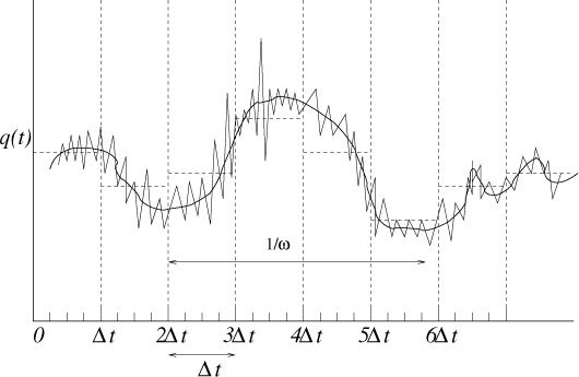
Figure 4-2. Coarse graining of different representations of a pattern changing in time: the actual detailed signal (jagged line), smoothed into a trend (smooth curve), and then re-digitized into coarse blocks of width Δt.
This idea of separating out noise, is not really different from the way we handle any kind of detail, whether perceiving or building something. Imagine how you would depict a scene for someone: if you visually sketched or otherwise described the object, you would probably begin by drawing the main lines, the broad strokes of the image, and only then start to fill in details at lower levels. You would start from the top down in the scale hierarchy. However, if you tried to draw something like a lawn of grass, with thousands of detailed parts all the same, you would probably just start drawing the details one by one, because there would be no trend to identify. There would be nothing to gain from starting anywhere else, because there is not identifiable trend to extract. The half-closed eye test allows us to see major trends and features in an image.
Trends are part of the way we perceive change, whether it is change in time or in space. It is common to decompose variation into something that is slowly varying that we want to see, and something else that is fluctuating on top of it that we don’t (see Figure 4-2). It is a common technique in mathematics, for instance: it is the basis of Fourier analysis, and it is the basic method of perturbation theory. It is a property of weakly coupled (linear) systems that this decomposition of scales leads to a clear description of trends. In fact it is a property of the interference of waves. We can express it in a number of suggestive ways:
Change = Stable Variation + Perturbation |
Variable data = Trend + Variation |
Transmission = Signal + Noise |
In each case, the aim is to make the contributions on the right of the plus sign as small as possible.
Recall, for example, our love boat from Chapter 1, sailing on the calm ocean. At any particular zoom level, the picture of this boat had some general structural lines and some details that we would consider superfluous to the description. Viewed from the air, the picture was dominated by a giant storm, and then the ship was but a blip on the ocean. At the level of the giant waves, the ripples close to the ship were irrelevant details. At the level of the ripples, the atomic structure of the water was irrelevant, and so on.
Remember too that a small perturbation can unleash a self-amplifying effect in a non-linear system—the butterfly effect, from Chapter 1. If the small variations in Figure 4-2 did not average out to keep the smooth trend, but in fact sent it spinning out of control, then we would be looking at useless instability.
That is not to say that details are always unwelcome in our minds. Occasionally we are willing to invest the brute force to try to be King Canute in the face of an onslaught of detail. Perhaps the most pervasive trend in modern times is that we are including faster and faster processes, i.e. shorter and shorter timescales, in our reckoning of systems. We used to let those timescales wash over us as noise, but now we are trying to engage with them, and control them, because the modern world has put meaning there.
The fighter jet’s aerodynamic stability was one such example. Stock market trading prices are another where people actually care about the detailed fluctuations in the data. Traders on the markets make (and lose) millions of dollars in a split second by predicting (or failing to predict) the detailed movements of markets a split second ahead of time. Complex trading software carries out automated trading. This is analogous to the tactics of the fighter jet, to live on the brink of stability, assisted by very fast computers that keep it just about in the air, in a fine detailed balance at all times, modulo weekly variations. In most cases, however, we are not trying to surf on the turbulence of risk, we are looking for a safe and predictable outcome: something we can rely on to be our trusted infrastructure.
We now have a representation of change based on scales in space and time, and of rates of change in space and time. This is going to be important for understanding something as dynamic as information infrastructure. These two aspects (position and rate of change) are known as the canonical variables of a dynamical system. Let’s pursue them further.
As we zoom into any picture, we may divide it up into grains76, as in Figure 4-2, and imagine that the trend is approximately constant, at least on average, over each granular interval. The variations within the grain can thus be replaced by the flat line average of the values in the interval, for most purposes. If the grains are small enough (so that the size of Δt → 0), the result is that one smooths out the jagged fluctuations, leaving the smooth curve in the figure.
One may also do the same thing with the difference between the actual value and the average value. This gives us the average size of fluctuations, relative to that average base value in the grain. We can separate clarity and fuzz. The method does not work unless there is a separation of scale, however. If fluctuations are no smaller than the variations of a trend, then we can’t tell the difference between them, and the line is simply irreducibly jagged at all scales. This is called scale-free, self-similar, or even fractal behaviour. Dividing up a model into grains is also a strategy for computational modelling, but it does not work very well in non-linear systems, which is why it is hard to predict the weather (see Chapter 1).
Now back to information. Smoothing out fluctuations into a continuous curve is one approach to finding a stable representation of a process, but it is still varying continuously (or pseudo-continuously). What if we don’t make the grain size vanishingly small, but keep discrete grains or ‘buckets’? Then the value of the variation stays at the same fixed value for longer. This is a kind of quantization of the horizontal time axis. By removing detail, removing information, we actually find more meaning.
This idea can be used to exploit another approach called re-digitizing the signal. This is a way of sorting a signal into fixed symbol categories on the vertical axis (see Figure 4-3). This is where digital signal transmission comes back to us as a technology rather than as a discovery.
Recall that the telegraph used the clarity of digital Morse code to avoid the noisy transmission lines of the electrical wiring. By standardizing discrete units of time for dots and dashes, i.e. by digitizing the time for a dot, we can distinguish a dot from a dash in terms of a simple digital time scale. By setting a threshold between signal and no signal, a message of dots and the dashes could be distinguished as symbols from no message at all.
This same principle was applied both to the time axis and to the signal value, to digitize many other kinds of signal, starting from around the 1980s. What had previously been treated as continuous was cut up into a discrete template, or sampled (see Figure 4-3) so that it could be encoded as digits or symbols. Digital music resulted in the MiniDisc in Japan, and the Compact Disc (CD) all over the world. Video discs, DVDs and Blue-Ray followed. Now digital television and radio are the norm.
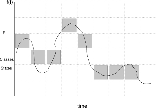
Figure 4-3. Re-digitization of the vertical axis an analogue signal is called A/D conversion. The rendition is not ‘perfect’, but we can make the symbol sensitivity as large or small as we like, so that variations within a digit do not matter.
Re-digitization brings stability to our perception of location on these maps of sound and picture: as long as a signal stays within the bounds of certain thresholds we have assigned, the digital representation records a specific symbol. Thus, if we divide up the ‘continuous’ signal values into coarse enough ranges, then the effect of noise will be almost unnoticeable, because it will be like moving a couple of blocks within the radius of the city. Our ears are not sensitive enough to detect the difference. A perturbation of the average signal will still be within the bounds of a category. This is the method of analogue to digital (A/D) conversion.
Harry Nyquist (1889-1976) made famous a theorem which tells us that, in order to capture the detail of a change in time, we have to sample the signal into buckets at least twice as fast as the fastest expected change. That is why digital music is represented in sampling rates of 44kHz (16 bits) and 48-192kHz (24 bits), as the highest frequencies available to human hearing are reckoned to be at most 20kHz. The higher quality sampling used by audiophiles is designed to capture more of the harmonics and interactions that happen during the reproduction of the music, even if the actual frequencies cannot be perceived directly.
Average behaviour seems to be a key to the way humans perceive change. I’ll return to this topic in the second part of the book. We can grasp trends over a limited range, and we ignore the fluctuations on a smaller scale. Thus our interaction and comprehension of a scene depends completely on how we set our scope. These matters are important when designing technology for human interaction, and they tell us about the sensitivity of machinery we build to environmental noise.
So let’s delve deeper into the balance of fluctuations, and consider what this new notion of stability means, based on the more sophisticated concept of averages and statistical measures. A change of setting might help.
Global warming and climate change are two topics that rose swiftly into public consciousness a few years ago, to remind us of the more tawdry concept of accounting and balancing the books. It took what had previously been a relatively abstract issue for meteorologists about the feedback in the global weather systems and turned it into a more tangible threat to human society. The alleged symptoms became daily news items, and pictures of floods, storms, and drowning polar bears became closely associated with the idea. Climate change is a new slogan, but it all boils down to yet another example of scaling and stability, but this time of the average, statistical variety.
The weather system of our planet is a motor that is fuelled primarily by sunlight. During the daytime, the Earth is blasted continuously by radiation from the Sun. The pressure of that radiation bends the magnetic field of the planet and even exerts a pressure on the Earth, pushing it slightly outwards into space. Much of that radiation is absorbed by the planet and gets turned into heat. Some of it, however, gets reflected back into space by snow and cloud cover. During the night, i.e. on the dark side of the globe, the heat is radiated back into space, cooling one half of the planet. All of these effects perturb the dynamical system that is the Earth’s climate.
As chemical changes occur in the atmosphere, due to pollution and particles in the atmosphere, the rates of absorption and reflection of light and heat change too. This leads to changes in the details that drive the motor, but these changes are typically local variations. They happen on the scales of continents and days.
Usually, there is some sense in which the average weather on the planet is more or less constant, or is at least slowly varying. We call the slow variation of the average patterns the climate and we call the local fluctuations the weather. By analogy with the other cases above, we could imagine writing:
Atmospheric evolution = Climate + Weather
and, even though the weather is far from being a linear thing, we might even hope that there is a sufficient stability in the average patterns to allow us to separate the daily weather from the climate’s long term variation.
It makes sense then that, in the debates of global warming, the average temperature of the planet is often referred to. This is a slightly bizarre idea. We all know that the temperature in Hawaii and the temperature in Alaska are very different most of the time, so temperature is not a uniform thing. Moreover, the retention of heat in the atmosphere is non-linear, with weather systems creating all manner of feedback loops and transport mechanisms to move heat around, store it and release it. Ocean currents, like the gulf stream, transport heat from a hot place to a cold place. The planetary climate system is as intricate as biology itself.
The average temperature somewhere on the planet is thus in a continuous state of re-evaluation. It changes, on the fly, on a timescale that depends on the scale of the region we look at. For the average temperature of the whole Earth to be unchanging, the various absorptions, reflections, and re-radiations would have to balance out, in a truly Byzantine feat of cosmic accounting. A net effect of zero means that for all the energy that comes in from the Sun, or is generated on the planet, the same amount of heat must leak away. Such a balance is called a state of equilibrium.
The word equilibrium (plural equilibria) is from the Latin aequilibrium, from aequus ‘equal’, and libra meaning a scale or balance (as in the zodiac sign). Its meaning is quite self-explanatory, at least in intent. However, as a phenomenon, the number of different ways that exist in the world for weighing measures is vast, and it is this that makes equilibrium perhaps the most important concept in science.
Once again, equilibrium is about scale in a number of ways. As any accountant knows, yearly profits and monthly cashflow are two very different things. You might make a profit over the year, and still not be able to pay your bills on a monthly basis. Similarly, planetary heat input and dissipation both on the short term and in the long term are two very different issues. Of global warming, one sometimes hears the argument that all the fuel that is burned on the Earth is really energy from the Sun, because, over centuries, it is the conversion of raw materials into living systems that make trees and oil and combustible hydro-carbons. Thus nothing Man does with hydrocarbons can affect the long-term warming of the planet, since all the energy that went into them came from the Sun. On the short term, however, this makes little sense, since the energy stored in these vast memory bank oil reserves can be released in just a few years by little men, just as the chemical energy it took to make a stick of dynamite can be released in a split second. The balance of energy in and out thus depends on your bank account’s savings and your spending. Timescales matter.

Figure 4-4. The detailed balance between two parts of a system showing the flows that maintain equilibrium. The balance sheet always shows zero at equilibrium, but if we look on shorter timescales, we must see small imbalances arise and be corrected.
The basic idea of an equilibrium can be depicted as an interaction between two parties, as in Figure 4-4. The sender on the left sends some transaction of something (energy, data, money) to the receiver on the right at some kind of predictable average rate, and the receiver absorbs these transactions. Then, to maintain the balance, the roles are also reversed and the sender on the right transmits at an equivalent rate to the receiver on the left. The net result is that there is no build up of this transacted stuff on either side. It is like a ball game, throwing catch back and forth, except that there are usually far more transactions to deal with. In the case of global climate patterns there are staggering numbers of molecules flying back and forth in the atmospheric gases, transferring heat and energy in a variety of forms, and there are clouds and ocean currents transporting hot and cold water.
Equilibrium is what we observe when the slowly varying part of information grinds to a halt and becomes basically constant, so that one may see balance in the fluctuations. Equilibrium can be mechanical or seemingly static77, like when a lamp hangs from the ceiling, held in balance between the cord it is attached to and the force of gravity, or it can be more dynamic, such as the heating of the Earth, or a monthly cashflow, with a continuous input and output of income and expenses. (Imagine putting a group of people on a very large balance and weighing them first standing still, and then jumping up and down.) When an equilibrium is disturbed, the shift perturbs a system and this can lead to instability. Sudden destabilization catastrophes can occur, leading to new metastable regimes, like ice ages, microclimates, and other things. Equilibrium of discrete informatic values is often called the consensus problem in information science78.
Equilibrium might be the single most important idea in science. It plays a role everywhere in ‘the accounting of things’. It is crucial to our understanding of heat, chemistry, and economics—and to the Internet.
Although the simple depiction of equilibrium in Figure 4-4 shows only two parties, equilibrium usually involves vast numbers of atomic parts, taken in bulk. That is because equilibrium is a statistical phenomenon—it is about averages, taken over millions of atoms, molecules, data, money, or whatever currency of transaction we are observing. Staying in town, or quivering in your shoes are also statistical equilibria.
The accounting that leads to equilibrium is called a situation of detailed balance. It is detailed, because we can, if we insist, burrow down into the details of each individual exchange of atoms or data or money, but it is the balance over a much larger scale that is the key. The principle of detailed balance was introduced explicitly for collisions by Boltzmann. In 1872, he proved his H-theorem using this principle. The notion of temperature itself comes from a detailed balance condition.
A simple example of detailed balance is what happens in a queue. Recall the supermarket checkout example in Chapter 2. Customers arrive at a store, and they have to leave again, passing through the checkout. It seems reasonable to expect that this would lead to an equilibrium. But what if it doesn’t? What if more customers arrive than leave? When a sudden change in this equilibrium happens, the balance of flows is affected and the detailed balance goes awry until a new stable state is reached. This is a problem for non-equilibrium dynamics. However, often we can get away without understanding those details, by dealing only with the local epochs of equilibrium, in the pseudo-constant grains of Figure 4-2.
Queueing theory begins with a simple model of this equilibrium that represents the arrival and processing of customers to a service handling entity, like a store, a call centre, or form-processing software on the Internet. In the simplest queueing theory, one imagines that customers arrive at random. At any moment, the arrival of a new customer is an independent happening, i.e. it has nothing to do with what customers are already in the queue. We say that the arrival process has no memory of what happened before. This kind of process is called a Markov process after Russian mathematician Andrey Markov (1856-1922), and it is a characteristic signature of statistical equilibrium. An equilibrium has no memory of the past, and no concept of time. It is a steady state.
Queueing theory can be applied by setting up the detailed balance condition and solving the mathematics. In normal terminology, we say that there is a rate of customers arriving, written λ requests per unit time, and there is a rate at which customers are served, called μ requests per unit time. From dimensional analysis, we would expect the behaviour of the queue to depend on the dimensionless ratio called the traffic intensity,

as indeed it does. To see that, we write the detailed balance as follows. A queue of length n persons will not be expected to grow or shrink if:
Expected arrivals = Expected departures
Or, as flow rates:
λ× (Probability of n – 1 in queue) = μ× (Probability of n in queue)
This says that, if a new person arrives when there are already n – 1 persons in line, it had better balance the rate at which someone leaves once there are now n persons in line. This detailed balance condition can be solved to work out an average queue length that can be supported, based on the dimensionless ratio ρ:

A picture of the results of this average length can be seen in Figure 4-5, and they are quite intuitive. As long as the arrival rate of customers is a bit less than the rate at which customers can be processed, ρ is less than the dimensionless number 1 and the queue length is small and under control. However, there is a very critical turnaround as one scale approaches the other, sending the queue into an unstable mode of growth. The suddenness of the turning point is perhaps surprising. The queue has a major instability, indicating that we should try to keep queues small at all times to avoid a total breakdown. Indeed, after a half century of queueing theory, the crux of what we know is very simple. A queue has basically two modes of operation. Either the expected queue length is small and stable, or it is growing wildly out of control—and the distance between these two modes is very small.
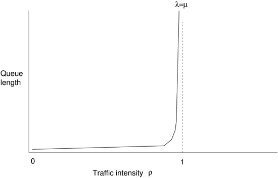
Figure 4-5. The behaviour of the average queue length predicted by a detailed balance relation in queueing theory. The queue goes unstable and grows out of control when ρ → 1. theory
The model above is completely theoretical, but since it is based mainly on simple scaling assumptions, we would expect it to represent reality at least qualitatively, if not quantitatively. For computer processing, queueing is a serious issue, that affects companies financially when they make legal agreements called Service Level Agreements, claiming how fast they can process data requests. Companies need to invest in a sufficient number of servers at the ‘data checkout’ of their infrastructure to process arrivals in time.
In 2007, together with students Jon Henrik Bjørnstad, Sven Ulland and Gard Undheim, I studied how well this very real issue is represented by the simple model above, using real computer servers. For all the wonders of mathematics and modelling, simplicity is an asset when building technology, so we wanted to know if a simplest of arguments would provide good-enough guidance to datacentre infrastructure designers. The results can be seen in Figure 4-6 and Figure 4-7.
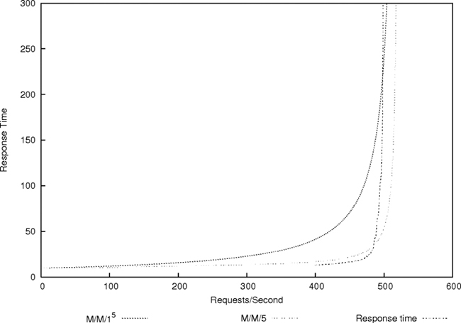
Figure 4-6. Queue behaviour of five servers in different configurations, comparing the two models with measurements.
The different lines in Figure 4-6 show the same basic form as the theoretical graph in Figure 4-5, indicating that the basic qualitative form of the behaviour is quite well described by the simple model, in spite of many specific details that differ79. This is an excellent proof of the universality of dimensional arguments based on scaling arguments.
Figure 4-6 also shows the different ways of handling requests. The experiment was set up with five servers to process incoming online requests. Queueing theory predicts that it makes a difference how you organize your queue. The optimum way is to make all customers stand in one line and take the first available server from a battery of five as they become available (written M/M/5). This is the approach you will see at airports and other busy centres for this reason. The alternative, is to have a separate line for each sever (written M/M/15). This approach performs worse, because if the lines are not balanced, more customers can end up in a busy line, while another line stands empty. So we see, from the graph, that the single line keeps faster response times much closer to the critical turning point than the multiple-line queue, which starts going bad earlier—but both queue types fail at the same limit.
Unlike the simple theory, we can also see how the finite capacity of the computer eventually throttles the growth of a queue (another dimensionless ratio), illustrating where the simple model of scale and balance breaks down. Compare Figure 4-5 with Figure 4-7. When the response time was modelled in detail to find the limit, we see that the response time does not actually become infinite, because the computer cannot work that hard. In fact what happens (compare the two overlaid lines in Figure 4-7) is that when the queue length is so long that the CPU cannot process the requests any faster (ρ → 1), the computer becomes immobilized by its own inundation with work and it begins to drop jobs. This situation is called thrashing. The computer loses the ability to focus on processing jobs and so its average CPU utilization actually falls, as the jobs are still building up. The vertical bars, showing the statistical variation in repeated experiments, show how the processor becomes very unpredictable. It copes about half of the time to do useful work, and the response time of the few jobs that get done reaches a maximum limit.
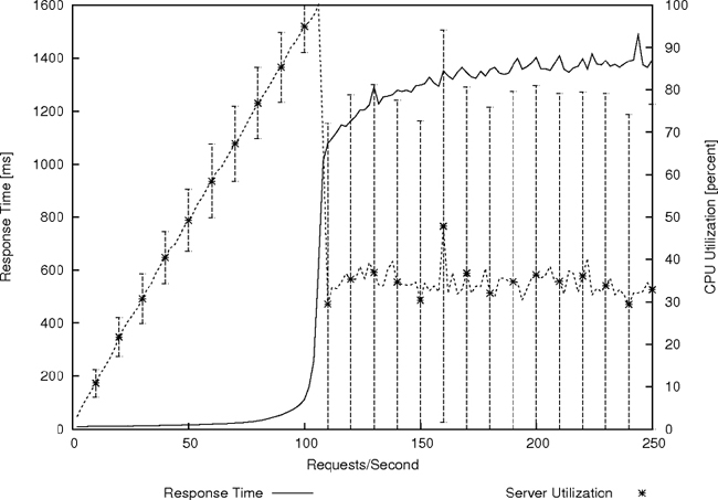
Figure 4-7. Two overlaid graphs showing the CPU utilization and the response time of a server depending on the arrival rate of requests. The utilization is a straight line up to saturation at ρ = 1 and then it actually falls as the system goes chaotic. The response time rises to a maximum value at around 1300 ms and stabilizes due to the finite scale of resources in the computers.
The simple M/M/5 model did not take into account the characteristic limiting scales of the computers so it was always ready to fail once that assumption was violated. Before this point was reached, on the other hand, the main features of the behaviour were still very well modelled by it.
The expectation that equilibrium would be important to computer behaviour had been one of my chief lines of reasoning in the paper, Computer Immunology, when I wrote about self-healing computer systems even as early as 1998, because it is such a universal phenomenon, but I had not then had time to think in detail about what kind of equilibria might be important. It seemed therefore important to gain a broad understanding of the kinds of phenomena taking place in the world of computer based infrastructure.
Beginning in 1999, and working with colleagues Hårek Haugerud, Sigmund Straumsness, and Trond Reitan at Oslo University College, I began to apply the technique of separating slow and fast variables to look at the behaviour of different kinds of service traffic (queues) on computers that were available to us. I was particularly interested in whether the standard methods of statistical physics could be applied effectively to describe the pieces of technological wizardry being used at a different scale. Dynamical similarity suggested that this must be the case, but idealizations can sometimes go too far. To what extent would it be possible to make simple idealized models as in Newtonian physics?
We began by measuring as many of the facets of computer behaviour as we could, over many months, to see what kinds to phenomena could be identified. Collecting numbers is easy, but piecing together an understanding of what they mean is another matter altogether. This is the first stage of any scientific investigation: look and see80.
The initial investigations were less than interesting. Merely collecting data is no guarantee of striking gold, of course. We began by looking at a group of computers used by the staff at the university on their desktops. They were readily available and so setting up the experiment was quite easy. However, the data returned were both sparse and hard to fathom. If you imagine, for a moment, the life of a typical desktop computer, it is more like a cat than a ballet dancer: it sleeps for a lot of the time, we feed it now and then, but there are no sweeping patterns of regular activity that could be used to infer some larger theme, worthy of even the most paranoid scrutiny.
Desktop and laptop computers, it turns out, are very wasteful of the quite generous resources they sport. We almost never utilize their potential for more than a small percentage of the time they are switched on. We shouldn’t expect to see any fathomable pattern from a single computer, over a timescale of its usage. Most of that time they merely sit idle, waiting for something to do.
A negative result is still a result, though. Knowing what can cannot be known is an important part of science: fundamental uncertainty, somewhat analogous to the quantum world, where the behaviour of individual quanta is truly uncertain, but where patterns emerge on average at much larger scales. Indeed, as we moved on to explore ‘servers’ (these are the computers that handle what happens when you look up something online, for example, like web pages and database items), basic patterns of behaviour revealed themselves quite quickly. In fact, we could see two kinds of system: those where very little happened and dominated by random noise, and those with clear patterns of periodic activity. Computers that were used by just a single user from time to time, like workstations and PCs were dominated by noise, because when so little actually happens, everything the user did was new and apparently random. Busy servers, on the other hand, servicing hundreds or thousands of users, showed clear statistical patterns of repeated behaviour.
Classical computer science would have us believe that computers are just machines and therefore they can only do what they have been told to do, slavishly following a particular path. However, this is manifestly not the case. It’s a bit like saying that if the Sun is shining, it must be sunny—that is too simplistic (clouds still get in the way, even if the sun is shining, for instance). Even when we had found enough data from busy servers to see recognizable patterns, there were things that defied the classical explanation of a deterministic system.
Overlapping timescales were one such mystery. When you know that a certain task is executed at a certain moment by a computer, you might expect to see a clear signature from this task, but that is also too simplistic. The more we looked for signs of specific deterministic behaviour in the measurements, the less of a pattern we actually saw. It was almost as if the computer’s response to individual behaviour was doing the exact opposite of what one would expect. It was surprisingly stable and seemed to be more of a mirror for our circadian rhythms than our intentions. Immediate human intent was the farthest thing from what we were seeing.
The mystery deepened when the ‘auto-correlation’ time of signals was longer than the variations in the trends we were observing. A correlation is a similarity in a pattern of measurement at two different places (in space). An autocorrelation is a correlation at two different times (in time). It represents the appearance of a memory in what otherwise looked like quite random data. Computers were not Markov processes.
But in fact the problem was neither paradoxical nor counter-intuitive. The problem lay in trying to look for channels of determinism in measurements that were overlapping to such a high degree that the signals of individual contributions were averaged out—or coarse grained away (as in Figure 4-2). All that remained of the signal was the slowly varying trend. What we were looking at was no longer a deterministic machine, but a non-equilibrium body immersed in a bath of environmental chatter. We were seeing clear patterns that were dominated by the human working week (see Figure 4-8).
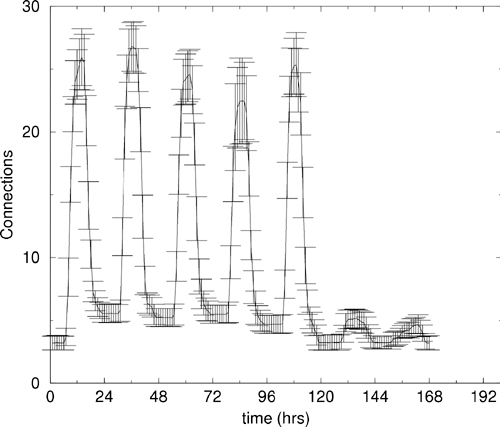
Figure 4-8. Measured data from a Samba file access services, measured over many weeks, plotted overlapping onto a single week. Vertical bars represent the variation of the measurements. The fact that the error bars are small compared to the scale of variation, shows this to be a strong signal with little noise.
On single-user machines, users’ behaviours became the loudest message in the flood of environmental signals. The behaviour looked unpredictable, because user behaviour is basically unpredictable when viewed on a one by one basis. First you type some letters, then you make a cup of coffee, then you type some more into a different application, then you are interrupted by a colleague. On this individual basis, there is a strong coupling between user and machine, making it difficult to see any long term behaviour at a separate scale; but, once a machine is exposed to many users (the more the better, in fact) all of those specific details interfere and details smudge out the fluctuations leaving only the trend.
Once we saw how the dynamics were being generated, it led to some obvious ways to unite theory and practice. The strong periodic behaviour first suggested that we should model the system using periodic variables. The mathematics of Fourier analysis then make the prediction that the effective contributions to system behaviour will be quantized in integer multiples, just like the energy levels in quantum blackbody radiation.
Moreover, the strong periodicity suggested that, if we subtracted the emergent trend from the rest of the signal, by separating fast and slow variables, what would be left should look like an equilibrium distribution, with periodic boundary conditions, much like Planck radiation. Sure enough, when we did this, out popped a beautiful picture of the Planck spectrum81.
It is important to understand why the spectrum of fluctuations in our computer systems matched the quantum radiation signature of blackbody radiation. There is nothing quantum mechanical about computer behaviour at the scale of desktops and servers. However, the periodicity of the environmental driving factors effectively led to a system that was dynamically similar, and similar systems have similar behaviour. The conclusion is that computers are, in fact, in effective equilibrium with their surroundings at all times, with regard to their network connections, just as the Earth is in equilibrium with outer space.
What was perhaps more important than the dynamical similarity was that one could immediately see that computers were not to be understood as something operating independently of humans. They are not just machines that do what they are told: it is all about understanding a human-computer system82. The message visible in the non-equilibrium pattern gave us strong information about the source that drives the trends of change.
This is not mysterious either. Computers do indeed do more or less what we tell them, but what we tell them is only one message amongst many being received and processed by a modern computer. There are multiple overlapping messages from software, from the keyboard, the mouse, the network, and all of these are overlapping and interfering with one another. The difference is quite analogous to the transition from the picture of a Newtonian particle as a point-like ball moving in a straight line, to a spritely quantum cloud of interfering pathways, as revealed by Feynman’s diagrams.
In looking at a small web server, we observed that we needed to have a minimum amount of traffic to the server in order to be able to see any pattern on the time scale of weeks. This revealed a periodic pattern on the scale of a week. My team was unable to go beyond this stage, but online retailer Amazon took this to the next level in the early years of the 21st century. Amazon web traffic is vast.
With traffic intensity and levels tens of millions of times greater than our lowly web server, and data collection over years, it was possible to see a pattern on an even greater scale of yearly patterns.
Amazon’s sales are fairly steady throughout the year, except at the time leading up to Christmas, when sales suddenly rise massively. Extra information processing capacity is needed to cope during these months. This is no different to the need to hire extra sales personnel for the Christmas period, in more traditional store, just on a much greater scale. Amazon builds extra capacity to cope with this sudden demand each year, and rents out the surplus during the rest of the year.
The growth of Amazon’s traffic is so large that there no sense in which we can think of it as an equilibrium system over several years. What is interesting however is that the identification of the trend pattern has similarities that still make it somewhat predictable. This kind of knowledge enables Amazon to buy datacentre capacity at the level needed for the Christmas peak, but then rent it out to other users throughout the year. This was the start of ‘cloud computing’, using scale and detailed balance as a tool to spread the balance of costs.
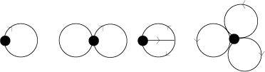
Figure 4-9. The quantum loop expansion—all the ways of staying in the same place
To predict the emergence of a Planck spectrum in weekly computer behaviour, I used the same trick that Feynman and Schwinger had used of summing up contributions of cause and effect in the development of QED. Closing the loop on the QED story illustrates yet again the generic structure of information transfer that underpins disparate phenomena. Based on the methods developed by Schwinger and students after the seminal work on QED, it is possible to see the signature of equilibrium visually, in a much broader context with the help of Feynman diagrams. The juxtaposition is fitting, as the work of Feynman and Schwinger have reached a kind of equilibrium of their own in modern times. The so-called effective action in quantum field theory is the generator of equilibrium processes in quantum field theory. Schwinger referred to this as merely a ‘generating functional’ for calculating particle processes. Feynman’s interpretation might have been more visual. Today, the effective action summarizes what is known as the quantum loop expansion, and it is known to be related to the free energy for equilibrium thermodynamics.
The significance of the effective action is that it generates all closed-loop diagrams and hence it represents the sum of all processes during which a ‘particle’, ‘message’, or ‘transaction’ (take your pick) is in balance with a counter-process so that the system goes nowhere at all. It sums up all the roads to nowhere. At equilibrium, for every message forwards, there is one backwards. These are the basic diagrams of an equilibrium, generalizing Figure 4-4.
In complete equilibrium there is no notion of time in a system, because we cannot observe any change of state. In fact, the notion of time disappears altogether.
Discovering the well-known science of equilibria in the statistical behaviour of information technology was a welcome opportunity to see modern infrastructure in a new light. For the first time, one could begin to develop a physics of the technology itself, to really begin to understand it behaviourally, in all its complexity, without oversimplifying or suppressing inconvenient issues.
Equilibrium presents itself in many flavours, important to technology, and this chapter could not call itself complete without mentioning more of the practical applications of equilibria. What one learns from the loops above is that a state of equilibrium is always a place from which to begin generating an understanding of dynamics, because it represents a state in which nothing actually happens on average, but which is poised to unleash anything that is possible by perturbing.
Consider the climate analogy again. The net warming of the planet is not the only manifestation of disequilibrium in climate change. The increased energy from warming causes more water to evaporate from the oceans and then more precipitation to fall over land. This is a sub-part equilibrium around water. Rain and snow pour greater and greater amounts of water onto land, causing flooding in many areas. Why flooding? Flooding occurs because drainage systems cannot cope with the amount of water falling, so rivers burst their banks and irrigation/drainage channels become super-saturated in their attempt to return water to the sea: a broken equilibrium. The same effect happens with Internet traffic, but it is harder to visualize.
Flooding seems to be worse in recent years, and it has been speculated whether this is due to poor drainage in farmland. Drainage, of course, is not a natural phenomenon; it is one of our human infrastructure technologies for maintaining an artificial equilibrium. If drainage is designed during a time of little precipitation, it is tempting for the engineers to dimension their system for a capacity on the same scale as the average levels of rainfall over recent years. No one builds for the hundred year flood, because that does not make short term cashflow sense. Unlike Amazon, drain builders cannot monetize their peak load investments by renting out spare drainage capacity during the times of low rainfall. This makes the boundary between land and water unstable to rainfall, because it cannot be equilibrated.
We can understand the key features of this instability easily by looking at Figure 2-1 again, with a slightly different focus. The left hand picture, which was stable to the location of the ball, has a beneficial effect to perturbations like the wind that pushes it around; but it has a harmful effect if your perturbation is the arrival of new balls, like raindrops, for then we see that containing these causes the valley to fill up and flood. This has to happen on a timescale determined by the size of the valley and the rate of rainfall.
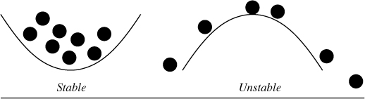
Figure 4-10. A valley is unstable to filling with raindrops, but a hill is stable.
The right hand picture, which is unstable to ball position and motion, now becomes the perfect drainage system, keeping it free of flooding. Thus the roles of the potential are reversed with respect to the two different kinds of perturbation.
This situation is very interesting from a technological perspective, because we have discovered something new to the discussion thus far, namely a conflict of interest in the design of a system. We need a mechanism to support two different goals, and we find that it cannot necessarily do so, at least without redesign.
Suppose you are a technology designer, or infrastructure engineer, with the responsibility to build a safe and practical solution to keep animals safe and contained. You might consider making a confining potential to keep the animals from wandering off, and you might not consider the possibility that flooding might have placed these animals in the perfect trap where they would drown. There is thus a design conflict between containment and filling up with water.
Now, if water is allowed to drain out of the potential valley above, by making a hole, say, one could try to change the unstable growth into a manageable equilibrium. Then we introduce a new scale into the problem: the size of the hole, or the rate at which water drains from the valley.
In fact, the very same conflict exists in many cities where insufficient planning is made for drainage. In some towns where there is rarely rain, there are no storm drains at all, and water has to flow across concrete and asphalt roads causing flooding. In my home city of Oslo, Norway, snow often builds up in winter and snow ploughs pile the snow on top of storm drains so that, when the snow begins to melt, the drains are blocked and the streets flood. Buildings with flat rooves with walls around them have a similar problem: water builds up on the roof and does not drain away properly, causing leakage through the ceiling below.
Conflicts of interest between design goals may be considered part of a more general problem of strategic decision-making, a topic that has been analyzed extensively by mathematicians during the 20th century. The subject is also known as game theory.
John von Neumann, whom we met in the previous chapter, was one of the earliest innovators in game theory. He discovered the solution to the now famous concept of zero sum games, a kind of game in which what one player loses, the other player gains. Game theory developed over the 20th century to be a key consideration in formulating problems of economics. Indeed, von Neumann’s seminal book with economist Oskar Morgenstern (1902-1977) is considered by many to be the birth of modern economics83.
A zero sum game is a game with conservation of rewards, i.e. where there is a fixed amount of benefit to share amongst everyone. This is like the accounting of energy in physics, or a scenario in which there is a fixed amount of money to go around. Although we can make games with any number of players, it is easiest to imagine two opposing players in a tug of war, each competing to maximize their share of the reward. The reward is referred to as the payoff in game theory.
Suppose, for example, we think of the water sharing problem again: only a fixed amount of rain falls on an oasis in the desert. It is captured in a tank and we want to use it for a variety of different and conflicting purposes. One competing player wants to use the water to drink, another wants to use it to grow food. The water here is itself the payoff, and the players pursue a tug of war to maximize their share of the water. If one player gets 2 litres, the other player loses those 2 litres, hence the sum of the payoffs is zero.
The idea in game theory is that both players, or stakeholders formulate their strategies, possibly several different ones, in order to maximize their use of the water. We can then evaluate which strategy would give each player a maximum payoff, given that the other player is trying to do the very same thing. It is a tug of war.
Von Neumann used the concept of an equilibrium to formulate a solution to this kind of game. He showed that one could make a detailed balance condition for the payoff known as the minimax condition, where one balances the combination of minimum payoff for an opponent with the maximum payoff for oneself. The minimax detailed balance looks deceptively simple:

but it is not very illuminating without delving into the detailed mathematics. Importantly, von Neumann was able to show that every zero sum game could be solved to find the optimum compromise for both parties in the case of the zero sum game. If there was detailed balance, each player may choose a single pure strategy to maximize their payoff. If the balance was broken, they could still find compromise, but only by playing a mixture of different strategies. This was called his minimax theorem.
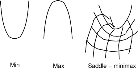
Figure 4-11. A minimax or saddle point is a maximum in one direction and a minimum in the orthogonal direction. The saddle point represents the compromise between the desire to maximize one variable and minimize another.
The minimax theorem was hailed as a triumph of rational thought, and encouraged strategists, especially during the Cold War, to spend time on optimal strategy computation. It applied equilibrium thinking to human motivated compromise, using only numbers for payoffs obtained from, at least in principle, a rational or impartial source. The limitation of zero sum was restrictive however. Not all situations are so clear cut about who wins and who loses. A more general scenario is the non-cooperative game, in which players each seek to maximize their own value, but the game is not necessarily zero sum anymore.
For example, suppose you are watching the television with your family, and everyone in the family has their own remote control (perhaps as an application on their smart phones). This might sometimes work in everyone’s favour. You might choose to work together, but you might also choose open conflict, changing the channel back and forth. Non-cooperative game theory asks: are there any solutions to this kind of scenario, in which everyone in the family maximizes their winnings? If this example sounds frivolous, consider an analogous scenario that is more serious.
Many of our technologies rely on sharing common resources amongst several parties, such as agricultural and grazing land, phone lines, electricity, water supplies, and computer networks, to mention just a handful. When we do this, we are aware that there will be contention for those resources—a tug of war, but not necessarily a zero sum game. Consider two examples that have a similar character. Imagine first that you are staying in a hotel. The hotel has limited space and can choose to give every customer either a tiny private bathroom with a ration of hot water, or a common bathroom with the same total amount of water and more space. The common bathroom would be much more luxurious and the experience would be superior, with more hot water available and more space, provided not many customers tried to use it at the same time. We could say that, as long as bathroom traffic was low, the common bathroom would be superior. However, when traffic becomes high, the private bathroom is preferred because customers then know that they will always get their fair share, even when that fair share is very small.
The same scenario could be applied to sharing of drains and sewers that might be blocked in a developing community. It also applies to the data networks that are spreading all over the planet. Two kinds of technology for network sharing exist: free-for-all sharing technologies like Ethernet and WiFi, which correspond to the common bathroom, and private line technologies like ATM, MPLS or cable modems, which correspond to the private bathroom84. If you are lucky and you are using a common wireless, the experience can be very good and easy, but when many users try to use it at the same time, you no longer have the experience of a fair share. Indeed, when the more users try to share, fewer actually get a share because a lot of time is wasted in just colliding with one another. Thus what is lost by one is not necessarily gained by another. This is not a zero sum game: it is worse.
The scenario was called the Tragedy of the Commons by ecologist Garrett James Hardin (1915-2003)85, and is often cited as an example of contention for shared resources. In economics, and indeed politics, the same situation occurs in bargaining for something, and it had long been recognized that the work of Morgenstern and von Neumann did not adequately address this issue.
A formulation of this problem was found by mathematician John Nash (1928-), when he was still an undergraduate at Princeton in 194986. Nash was eager to work with von Neumann on the issues of game theory, and went to some lengths to show him a proposed solution, but von Neumann was dismissive of the idea, busy with his many projects and consulting engagements and had little time for undergraduates. Nash was encouraged nevertheless by another mathematician and economist David Gale (1921-2008) and his work was published in the monthly proceedings of the National Academy of Sciences. Nash used a similar notion of equilibrium, called the Kakutani fixed point theorem, based not on single solutions but on mixtures of solutions (see Figure 4-12).
He showed that it was possible to find sets of strategies, in all cases, that would lead to an optimum outcome for mixed strategies. A Nash equilibrium is simply a stalemate in which no player can improve his or her position by changing strategy—the detailed balance of trying to maximize individual payoff could be solved. Nash showed that, for a very large category of games, such a solution had to exist. Since it was a generalization of the minimax theorem, it has largely superceded it today, and has become the de facto approach to looking for solutions in game theory87.
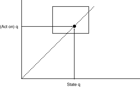
Figure 4-12. Fixed points are equilibria between the input and output of an operation that acts on input (horizontal axis) and produces an output (vertical axis). An equilibrium where (Act on) q = q must lie on the dotted line. In minimax a single match can be found. In the Nash equilibrium, sets of solutions that intersect the diagonal can satisfy the fixed point condition.
The Nash Equilibrium, as it is now known, has had an enormous impact on our understanding of subjects as wide as economics, evolutionary biology, computation and even international affairs88. It can be applied to policy selection in the continuum approximation, but not necessarily in a discrete system.
Fixed points are equilibria, and thus they are starting points for building stable systems. If we could construct technologies whose basic atoms only consisted of such fixed points, it would be a strong basis for reliability. No matter how many times the operation was applied, it would always stabilize. It turns out that we can, in many cases.
It is possibly ironic that an understanding that powered the dirty industrial age of steam should share so much with that which is powering the pristine information age. Harnessing equilibrium for constructive, predictable control of change, we can conquer many frontiers of interaction, from machinery to chemistry, biology, decision making, maintenance and even information. Dynamical similarity works in mysterious ways, yet it is the nature of this form of dynamic stability that brings a universality to our understanding of it. It means we can be confident that such simple minded arguments are still at the heart of phenomena across all areas of technology.
Get In Search of Certainty now with the O’Reilly learning platform.
O’Reilly members experience books, live events, courses curated by job role, and more from O’Reilly and nearly 200 top publishers.

