High Performance Python

Chapter 1. Understanding Performant Python

Programming computers can be thought of as moving bits of data and transforming them in special ways in order to achieve a particular result. However, these actions have a time cost. Consequently, high performance programming can be thought of as the act of minimizing these operations by either reducing the overhead (i.e., writing more efficient code) or by changing the way that we do these operations in order to make each one more meaningful (i.e., finding a more suitable algorithm).

Let’s focus on reducing the overhead in code in order to gain more insight into the actual hardware on which we are moving these bits. This may seem like a futile exercise, since Python works quite hard to abstract away direct interactions with the hardware. However, by understanding both the best way that bits can be moved in the real hardware and the ways that Python’s abstractions force your bits to move, you can make progress toward writing high performance programs in Python.

The Fundamental Computer System

The underlying components that make up a computer can be simplified into three basic parts: the computing units, the memory units, and the connections between them. In addition, each of these units has different properties that we can use to understand them. The computational unit has the property of how many computations it can do per second, the memory unit has the properties of how much data it can hold and how fast we can read from and write to it, and finally the connections have the property of how fast they can move data from one place to another.

Using these building blocks, we can talk about a standard workstation at multiple levels of sophistication. For example, the standard workstation can be thought of as having a central processing unit (CPU) as the computational unit, connected to both the random access memory (RAM) and the hard drive as two separate memory units (each having different capacities and read/write speeds), and finally a bus that provides the connections between all of these parts. However, we can also go into more detail and see that the CPU itself has several memory units in it: the L1, L2, and sometimes even the L3 and L4 cache, which have small capacities but very fast speeds (from several kilobytes to a dozen megabytes). These extra memory units are connected to the CPU with a special bus called the backside bus. Furthermore, new computer architectures generally come with new configurations (for example, Intel’s Nehalem CPUs replaced the frontside bus with the Intel QuickPath Interconnect and restructured many connections). Finally, in both of these approximations of a workstation we have neglected the network connection, which is effectively a very slow connection to potentially many other computing and memory units!

To help untangle these various intricacies, let’s go over a brief description of these fundamental blocks.

Computing Units

The computing unit of a computer is the centerpiece of its usefulness—it provides the ability to transform any bits it receives into other bits or to change the state of the current process. CPUs are the most commonly used computing unit; however, graphics processing units (GPUs), which were originally typically used to speed up computer graphics but are becoming more applicable for numerical applications, are gaining popularity due to their intrinsically parallel nature, which allows many calculations to happen simultaneously. Regardless of its type, a computing unit takes in a series of bits (for example, bits representing numbers) and outputs another set of bits (for example, representing the sum of those numbers). In addition to the basic arithmetic operations on integers and real numbers and bitwise operations on binary numbers, some computing units also provide very specialized operations, such as the “fused multiply add” operation, which takes in three numbers, A,B,C, and returns the value A * B + C.

The main properties of interest in a computing unit are the number of operations it can do in one cycle and how many cycles it can do in one second. The first value is measured by its instructions per cycle (IPC),^[1] while the latter value is measured by its clock speed. These two measures are always competing with each other when new computing units are being made. For example, the Intel Core series has a very high IPC but a lower clock speed, while the Pentium 4 chip has the reverse. GPUs, on the other hand, have a very high IPC and clock speed, but they suffer from other problems, which we will outline later.

Furthermore, while increasing clock speed almost immediately speeds up all programs running on that computational unit (because they are able to do more calculations per second), having a higher IPC can also drastically affect computing by changing the level of vectorization that is possible. Vectorization is when a CPU is provided with multiple pieces of data at a time and is able to operate on all of them at once. This sort of CPU instruction is known as SIMD (Single Instruction, Multiple Data).

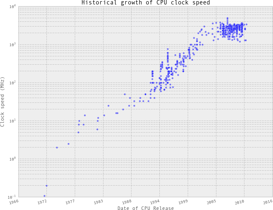
In general, computing units have been advancing quite slowly over the past decade (see Figure 1-1). Clock speeds and IPC have both been stagnant because of the physical limitations of making transistors smaller and smaller. As a result, chip manufacturers have been relying on other methods to gain more speed, including hyperthreading, more clever out-of-order execution, and multicore architectures.

Hyperthreading presents a virtual second CPU to the host operating system (OS), and clever hardware logic tries to interleave two threads of instructions into the execution units on a single CPU. When successful, gains of up to 30% over a single thread can be achieved. Typically this works well when the units of work across both threads use different types of execution unit—for example, one performs floating-point operations and the other performs integer operations.

Out-of-order execution enables a compiler to spot that some parts of a linear program sequence do not depend on the results of a previous piece of work, and therefore that both pieces of work could potentially occur in any order or at the same time. As long as sequential results are presented at the right time, the program continues to execute correctly, even though pieces of work are computed out of their programmed order. This enables some instructions to execute when others might be blocked (e.g., waiting for a memory access), allowing greater overall utilization of the available resources.

Finally, and most important for the higher-level programmer, is the prevalence of multi-core architectures. These architectures include multiple CPUs within the same unit, which increases the total capability without running into barriers in making each individual unit faster. This is why it is currently hard to find any machine with less than two cores—in this case, the computer has two physical computing units that are connected to each other. While this increases the total number of operations that can be done per second, it introduces intricacies in fully utilizing both computing units at the same time.

Figure 1-1. Clock speed of CPUs over time (data from CPU DB)

Simply adding more cores to a CPU does not always speed up a program’s execution time. This is because of something known as Amdahl’s law. Simply stated, Amdahl’s law says that if a program designed to run on multiple cores has some routines that must run on one core, this will be the bottleneck for the final speedup that can be achieved by allocating more cores.

For example, if we had a survey we wanted 100 people to fill out, and that survey took 1 minute to complete, we could complete this task in 100 minutes if we had one person asking the questions (i.e., this person goes to participant 1, asks the questions, waits for the responses, then moves to participant 2). This method of having one person asking the questions and waiting for responses is similar to a serial process. In serial processes, we have operations being satisfied one at a time, each one waiting for the previous operation to complete.

However, we could perform the survey in parallel if we had two people asking the questions, which would let us finish the process in only 50 minutes. This can be done because each individual person asking the questions does not need to know anything about the other person asking questions. As a result, the task can be easily split up without having any dependency between the question askers.

Adding more people asking the questions will give us more speedups, until we have 100 people asking questions. At this point, the process would take 1 minute and is simply limited by the time it takes the participant to answer questions. Adding more people asking questions will not result in any further speedups, because these extra people will have no tasks to perform—all the participants are already being asked questions! At this point, the only way to reduce the overall time to run the survey is to reduce the amount of time it takes for an individual survey, the serial portion of the problem, to complete. Similarly, with CPUs, we can add more cores that can perform various chunks of the computation as necessary until we reach a point where the bottleneck is a specific core finishing its task. In other words, the bottleneck in any parallel calculation is always the smaller serial tasks that are being spread out.

Furthermore, a major hurdle with utilizing multiple cores in Python is Python’s use of a global interpreter lock (GIL). The GIL makes sure that a Python process can only run one instruction at a time, regardless of the number of cores it is currently using. This means that even though some Python code has access to multiple cores at a time, only one core is running a Python instruction at any given time. Using the previous example of a survey, this would mean that even if we had 100 question askers, only one could ask a question and listen to a response at a time. This effectively removes any sort of benefit from having multiple question askers! While this may seem like quite a hurdle, especially if the current trend in computing is to have multiple computing units rather than having faster ones, this problem can be avoided by using other standard library tools, like multiprocessing, or technologies such as numexpr, Cython, or distributed models of computing.

Memory Units

Memory units in computers are used to store bits. This could be bits representing variables in your program, or bits representing the pixels of an image. Thus, the abstraction of a memory unit applies to the registers in your motherboard as well as your RAM and hard drive. The one major difference between all of these types of memory units is the speed at which they can read/write data. To make things more complicated, the read/write speed is heavily dependent on the way that data is being read.

For example, most memory units perform much better when they read one large chunk of data as opposed to many small chunks (this is referred to as sequential read versus random data). If the data in these memory units is thought of like pages in a large book, this means that most memory units have better read/write speeds when going through the book page by page rather than constantly flipping from one random page to another. While this fact is generally true across all memory units, the amount that this affects each type is drastically different.

In addition to the read/write speeds, memory units also have latency, which can be characterized as the time it takes the device to find the data that is being used. For a spinning hard drive, this latency can be high because the disk needs to physically spin up to speed and the read head must move to the right position. On the other hand, for RAM this can be quite small because everything is solid state. Here is a short description of the various memory units that are commonly found inside a standard workstation, in order of read/write speeds:

Spinning hard drive: Long-term storage that persists even when the computer is shut down. Generally has slow read/write speeds because the disk must be physically spun and moved. Degraded performance with random access patterns but very large capacity (terabyte range).
Solid state hard drive: Similar to a spinning hard drive, with faster read/write speeds but smaller capacity (gigabyte range).
RAM: Used to store application code and data (such as any variables being used). Has fast read/write characteristics and performs well with random access patterns, but is generally limited in capacity (gigabyte range).
L1/L2 cache: Extremely fast read/write write speeds. Data going to the CPU must go through here. Very small capacity (kilobyte range).

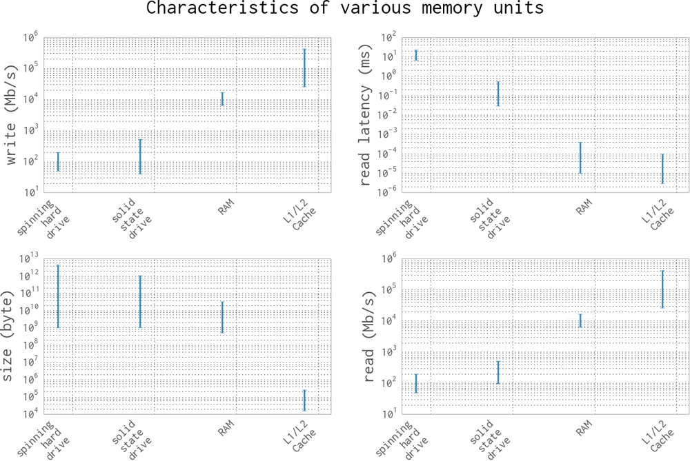
Figure 1-2 gives a graphic representation of the differences between these types of memory units by looking at the characteristics of currently available consumer hardware.

A clearly visible trend is that read/write speeds and capacity are inversely proportional—as we try to increase speed, capacity gets reduced. Because of this, many systems implement a tiered approach to memory: data starts in its full state in the hard drive, part of it moves to RAM, then a much smaller subset moves to the L1/L2 cache. This method of tiering enables programs to keep memory in different places depending on access speed requirements. When trying to optimize the memory patterns of a program, we are simply optimizing which data is placed where, how it is laid out (in order to increase the number of sequential reads), and how many times it is moved between the various locations. In addition, methods such as asynchronous I/O and preemptive caching provide ways to make sure that data is always where it needs to be without having to waste computing time—most of these processes can happen independently, while other calculations are being performed!

Figure 1-2. Characteristic values for different types of memory units (values from February 2014)

Communications Layers

Finally, let’s look at how all of these fundamental blocks communicate with each other. There are many different modes of communication, but they are all variants on a thing called a bus.

The frontside bus, for example, is the connection between the RAM and the L1/L2 cache. It moves data that is ready to be transformed by the processor into the staging ground to get ready for calculation, and moves finished calculations out. There are other buses, too, such as the external bus that acts as the main route from hardware devices (such as hard drives and networking cards) to the CPU and system memory. This bus is generally slower than the frontside bus.

In fact, many of the benefits of the L1/L2 cache are attributable to the faster bus. Being able to queue up data necessary for computation in large chunks on a slow bus (from RAM to cache) and then having it available at very fast speeds from the backside bus (from cache to CPU) enables the CPU to do more calculations without waiting such a long time.

Similarly, many of the drawbacks of using a GPU come from the bus it is connected on: since the GPU is generally a peripheral device, it communicates through the PCI bus, which is much slower than the frontside bus. As a result, getting data into and out of the GPU can be quite a taxing operation. The advent of heterogeneous computing, or computing blocks that have both a CPU and a GPU on the frontside bus, aims at reducing the data transfer cost and making GPU computing more of an available option, even when a lot of data must be transferred.

In addition to the communication blocks within the computer, the network can be thought of as yet another communication block. This block, however, is much more pliable than the ones discussed previously; a network device can be connected to a memory device, such as a network attached storage (NAS) device or another computing block, as in a computing node in a cluster. However, network communications are generally much slower than the other types of communications mentioned previously. While the frontside bus can transfer dozens of gigabits per second, the network is limited to the order of several dozen megabits.

It is clear, then, that the main property of a bus is its speed: how much data it can move in a given amount of time. This property is given by combining two quantities: how much data can be moved in one transfer (bus width) and how many transfers it can do per second (bus frequency). It is important to note that the data moved in one transfer is always sequential: a chunk of data is read off of the memory and moved to a different place. Thus, the speed of a bus is broken up into these two quantities because individually they can affect different aspects of computation: a large bus width can help vectorized code (or any code that sequentially reads through memory) by making it possible to move all the relevant data in one transfer, while, on the other hand, having a small bus width but a very high frequency of transfers can help code that must do many reads from random parts of memory. Interestingly, one of the ways that these properties are changed by computer designers is by the physical layout of the motherboard: when chips are placed closed to one another, the length of the physical wires joining them is smaller, which can allow for faster transfer speeds. In addition, the number of wires itself dictates the width of the bus (giving real physical meaning to the term!).

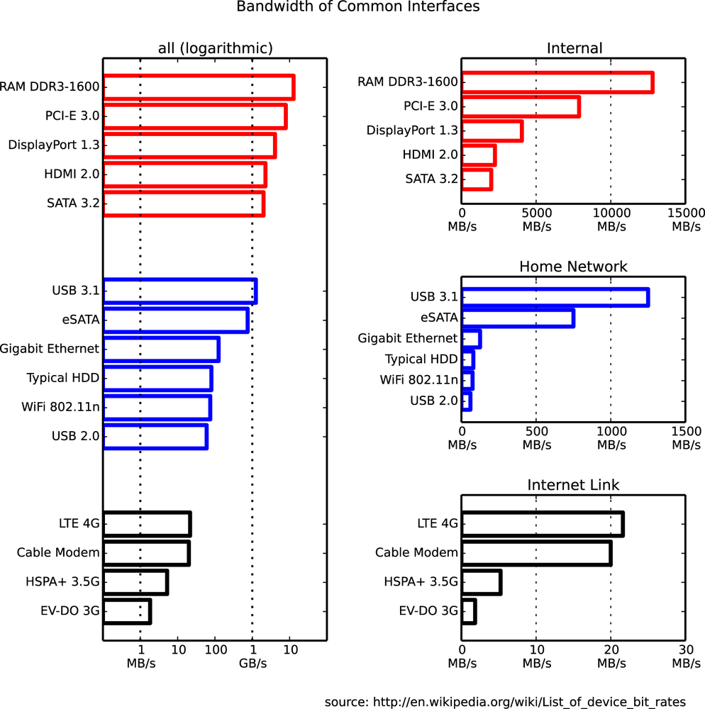
Since interfaces can be tuned to give the right performance for a specific application, it is no surprise that there are hundreds of different types. Figure 1-3 (from Wikimedia Commons) shows the bitrates for a sampling of common interfaces. Note that this doesn’t speak at all about the latency of the connections, which dictates how long it takes for a data request to be responded to (while latency is very computer-dependent, there are some basic limitations inherent to the interfaces being used).

Figure 1-3. Connection speeds of various common interfaces (image by Leadbuffalo [CC BY-SA 3.0])

Putting the Fundamental Elements Together

Understanding the basic components of a computer is not enough to fully understand the problems of high performance programming. The interplay of all of these components and how they work together to solve a problem introduces extra levels of complexity. In this section we will explore some toy problems, illustrating how the ideal solutions would work and how Python approaches them.

A warning: this section may seem bleak—most of the remarks seem to say that Python is natively incapable of dealing with the problems of performance. This is untrue, for two reasons. Firstly, in all of these “components of performant computing” we have neglected one very important component: the developer. What native Python may lack in performance it gets back right away with speed of development. Furthermore, throughout the book we will introduce modules and philosophies that can help mitigate many of the problems described here with relative ease. With both of these aspects combined, we will keep the fast development mindset of Python while removing many of the performance constraints.

Idealized Computing Versus the Python Virtual Machine

In order to better understand the components of high performance programming, let us look at a simple code sample that checks if a number is prime:

import math
def check_prime(number):
    sqrt_number = math.sqrt(number)
    number_float = float(number)
    for i in xrange(2, int(sqrt_number)+1):
        if (number_float / i).is_integer():
            return False
    return True

print "check_prime(10000000) = ", check_prime(10000000) # False
print "check_prime(10000019) = ", check_prime(10000019) # True

Let’s analyze this code using our abstract model of computation and then draw comparisons to what happens when Python runs this code. As with any abstraction, we will neglect many of the subtleties in both the idealized computer and the way that Python runs the code. However, this is generally a good exercise to perform before solving a problem: think about the general components of the algorithm and what would be the best way for the computing components to come together in order to find a solution. By understanding this ideal situation and having knowledge of what is actually happening under the hood in Python, we can iteratively bring our Python code closer to the optimal code.

Idealized computing

When the code starts, we have the value of number stored in RAM. In order to calculate sqrt_number and number_float, we need to send that value over to the CPU. Ideally, we could send the value once; it would get stored inside the CPU’s L1/L2 cache and the CPU would do the calculations and then send the values back to RAM to get stored. This scenario is ideal because we have minimized the number of reads of the value of number from RAM, instead opting for reads from the L1/L2 cache, which are much faster. Furthermore, we have minimized the number of data transfers through the frontside bus, opting for communications through the faster backside bus instead (which connects the various caches to the CPU). This theme of keeping data where it is needed, and moving it as little as possible, is very important when it comes to optimization. The concept of “heavy data” refers to the fact that it takes time and effort to move data around, which is something we would like to avoid.

For the loop in the code, rather than sending one value of i at a time to the CPU, we would like to send it both number_float and several values of i to check at the same time. This is possible because the CPU vectorizes operations with no additional time cost, meaning it can do multiple independent computations at the same time. So, we want to send number_float to the CPU cache, in addition to as many values of i as the cache can hold. For each of the number_float/i pairs, we will divide them and check if the result is a whole number; then we will send a signal back indicating whether any of the values was indeed an integer. If so, the function ends. If not, we repeat. In this way, we only need to communicate back one result for many values of i, rather than depending on the slow bus for every value. This takes advantage of a CPU’s ability to vectorize a calculation, or run one instruction on multiple data in one clock cycle.

This concept of vectorization is illustrated by the following code:

import math
def check_prime(number):
    sqrt_number = math.sqrt(number)
    number_float = float(number)
    numbers = range(2, int(sqrt_number)+1)
    for i in xrange(0, len(numbers), 5):
        # the following line is not valid Python code
        result = (number_float / numbers[i:(i+5)]).is_integer()
        if any(result):
            return False
    return True

Here, we set up the processing such that the division and the checking for integers are done on a set of five values of i at a time. If properly vectorized, the CPU can do this line in one step as opposed to doing a separate calculation for every i. Ideally, the any(result) operation would also happen in the CPU without having to transfer the results back to RAM. We will talk more about vectorization, how it works, and when it benefits your code in Chapter 6.

Python’s virtual machine

The Python interpreter does a lot of work to try to abstract away the underlying computing elements that are being used. At no point does a programmer need to worry about allocating memory for arrays, how to arrange that memory, or in what sequence it is being sent to the CPU. This is a benefit of Python, since it lets you focus on the algorithms that are being implemented. However, it comes at a huge performance cost.

It is important to realize that at its core, Python is indeed running a set of very optimized instructions. The trick, however, is getting Python to perform them in the correct sequence in order to achieve better performance. For example, it is quite easy to see that, in the following example, search_fast will run faster than search_slow simply because it skips the unnecessary computations that result from not terminating the loop early, even though both solutions have runtime O(n).

def search_fast(haystack, needle):
    for item in haystack:
        if item == needle:
            return True
    return False

def search_slow(haystack, needle):
    return_value = False
    for item in haystack:
        if item == needle:
            return_value = True
    return return_value

Identifying slow regions of code through profiling and finding more efficient ways of doing the same calculations is similar to finding these useless operations and removing them; the end result is the same, but the number of computations and data transfers is reduced drastically.

One of the impacts of this abstraction layer is that vectorization is not immediately achievable. Our initial prime number routine will run one iteration of the loop per value of i instead of combining several iterations. However, looking at the abstracted vectorization example, we see that it is not valid Python code, since we cannot divide a float by a list. External libraries such as numpy will help with this situation by adding the ability to do vectorized mathematical operations.

Furthermore, Python’s abstraction hurts any optimizations that rely on keeping the L1/L2 cache filled with the relevant data for the next computation. This comes from many factors, the first being that Python objects are not laid out in the most optimal way in memory. This is a consequence of Python being a garbage-collected language—memory is automatically allocated and freed when needed. This creates memory fragmentation that can hurt the transfers to the CPU caches. In addition, at no point is there an opportunity to change the layout of a data structure directly in memory, which means that one transfer on the bus may not contain all the relevant information for a computation, even though it might have all fit within the bus width.

A second, more fundamental problem comes from Python’s dynamic types and it not being compiled. As many C programmers have learned throughout the years, the compiler is often smarter than you are. When compiling code that is static, the compiler can do many tricks to change the way things are laid out and how the CPU will run certain instructions in order to optimize them. Python, however, is not compiled: to make matters worse, it has dynamic types, which means that inferring any possible opportunities for optimizations algorithmically is drastically harder since code functionality can be changed during runtime. There are many ways to mitigate this problem, foremost being use of Cython, which allows Python code to be compiled and allows the user to create “hints” to the compiler as to how dynamic the code actually is.

Finally, the previously mentioned GIL can hurt performance if trying to parallelize this code. For example, let’s assume we change the code to use multiple CPU cores such that each core gets a chunk of the numbers from 2 to sqrtN. Each core can do its calculation for its chunk of numbers and then, when they are all done, they can compare their calculations. This seems like a good solution since, although we lose the early termination of the loop, we can reduce the number of checks each core has to do by the number of cores we are using (i.e., if we had M cores, each core would have to do sqrtN / M checks). However, because of the GIL, only one core can be used at a time. This means that we would effectively be running the same code as the unparallelled version, but we no longer have early termination. We can avoid this problem by using multiple processes (with the multiprocessing module) instead of multiple threads, or by using Cython or foreign functions.

So Why Use Python?

Python is highly expressive and easy to learn—new programmers quickly discover that they can do quite a lot in a short space of time. Many Python libraries wrap tools written in other languages to make it easy to call other systems; for example, the scikit-learn machine learning system wraps LIBLINEAR and LIBSVM (both of which are written in C), and the numpy library includes BLAS and other C and Fortran libraries. As a result, Python code that properly utilizes these modules can indeed be as fast as comparable C code.

Python is described as “batteries included,” as many important and stable libraries are built in. These include:

unicode and bytes: Baked into the core language
array: Memory-efficient arrays for primitive types
math: Basic mathematical operations, including some simple statistics
sqlite3: A wrapper around the prevalent SQL file-based storage engine SQLite3
collections: A wide variety of objects, including a deque, counter, and dictionary variants

Outside of the core language there is a huge variety of libraries, including:

numpy: a numerical Python library (a bedrock library for anything to do with matrices)
scipy: a very large collection of trusted scientific libraries, often wrapping highly respected C and Fortran libraries
pandas: a library for data analysis, similar to R’s data frames or an Excel spreadsheet, built on scipy and numpy
scikit-learn: rapidly turning into the default machine learning library, built on scipy
biopython: a bioinformatics library similar to bioperl
tornado: a library that provides easy bindings for concurrency
Database bindings: for communicating with virtually all databases, including Redis, MongoDB, HDF5, and SQL
Web development frameworks: performant systems for creating websites such as django, pyramid, flask, and tornado
OpenCV: bindings for computer vision
API bindings: for easy access to popular web APIs such as Google, Twitter, and LinkedIn

A large selection of managed environments and shells is available to fit various deployment scenarios, including:

The standard distribution, available at http://python.org
Enthought’s EPD and Canopy, a very mature and capable environment
Continuum’s Anaconda, a scientifically focused environment
Sage, a Matlab-like environment including an integrated development environment (IDE)
Python(x,y)
IPython, an interactive Python shell heavily used by scientists and developers
IPython Notebook, a browser-based frontend to IPython, heavily used for teaching and demonstrations
BPython, interactive Python shell

One of Python’s main strengths is that it enables fast prototyping of an idea. Due to the wide variety of supporting libraries it is easy to test if an idea is feasible, even if the first implementation might be rather flaky.

If you want to make your mathematical routines faster, look to numpy. If you want to experiment with machine learning, try scikit-learn. If you are cleaning and manipulating data, then pandas is a good choice.

In general, it is sensible to raise the question, “If our system runs faster, will we as a team run slower in the long run?” It is always possible to squeeze more performance out of a system if enough man-hours are invested, but this might lead to brittle and poorly understood optimizations that ultimately trip the team up.

One example might be the introduction of Cython (Cython), a compiler-based approach to annotating Python code with C-like types so the transformed code can be compiled using a C compiler. While the speed gains can be impressive (often achieving C-like speeds with relatively little effort), the cost of supporting this code will increase. In particular, it might be harder to support this new module, as team members will need a certain maturity in their programming ability to understand some of the trade-offs that have occurred when leaving the Python virtual machine that introduced the performance increase.

^[1]Not to be confused with interprocess communication, which shares the same acronym—we’ll look at the topic in Chapter 9.

Get High Performance Python now with the O’Reilly learning platform.

O’Reilly members experience books, live events, courses curated by job role, and more from O’Reilly and nearly 200 top publishers.

Start your free trial

High Performance Python by Micha Gorelick, Ian Ozsvald