Chapter 1. Introduction
Before we start looking into all the moving parts of HBase, let us pause to think about why there was a need to come up with yet another storage architecture. Relational database management systems (RDBMSes) have been around since the early 1970s, and have helped countless companies and organizations to implement their solution to given problems. And they are equally helpful today. There are many use cases for which the relational model makes perfect sense. Yet there also seem to be specific problems that do not fit this model very well.[5]
The Dawn of Big Data
We live in an era in which we are all connected over the Internet and expect to find results instantaneously, whether the question concerns the best turkey recipe or what to buy mom for her birthday. We also expect the results to be useful and tailored to our needs.
Because of this, companies have become focused on delivering more targeted information, such as recommendations or online ads, and their ability to do so directly influences their success as a business. Systems like Hadoop[6] now enable them to gather and process petabytes of data, and the need to collect even more data continues to increase with, for example, the development of new machine learning algorithms.
Where previously companies had the liberty to ignore certain data sources because there was no cost-effective way to store all that information, they now are likely to lose out to the competition. There is an increasing need to store and analyze every data point they generate. The results then feed directly back into their e-commerce platforms and may generate even more data.
In the past, the only option to retain all the collected data was to prune it to, for example, retain the last N days. While this is a viable approach in the short term, it lacks the opportunities that having all the data, which may have been collected for months or years, offers: you can build mathematical models that span the entire time range, or amend an algorithm to perform better and rerun it with all the previous data.
Dr. Ralph Kimball, for example, states[7] that
Data assets are [a] major component of the balance sheet, replacing traditional physical assets of the 20th century
Widespread recognition of the value of data even beyond traditional enterprise boundaries
Google and Amazon are prominent examples of companies that realized the value of data and started developing solutions to fit their needs. For instance, in a series of technical publications, Google described a scalable storage and processing system based on commodity hardware. These ideas were then implemented outside of Google as part of the open source Hadoop project: HDFS and MapReduce.
Hadoop excels at storing data of arbitrary, semi-, or even unstructured formats, since it lets you decide how to interpret the data at analysis time, allowing you to change the way you classify the data at any time: once you have updated the algorithms, you simply run the analysis again.
Hadoop also complements existing database systems of almost any kind. It offers a limitless pool into which one can sink data and still pull out what is needed when the time is right. It is optimized for large file storage and batch-oriented, streaming access. This makes analysis easy and fast, but users also need access to the final data, not in batch mode but using random access—this is akin to a full table scan versus using indexes in a database system.
We are used to querying databases when it comes to random access for structured data. RDBMSes are the most prominent, but there are also quite a few specialized variations and implementations, like object-oriented databases. Most RDBMSes strive to implement Codd’s 12 rules,[8] which forces them to comply to very rigid requirements. The architecture used underneath is well researched and has not changed significantly in quite some time. The recent advent of different approaches, like column-oriented or massively parallel processing (MPP) databases, has shown that we can rethink the technology to fit specific workloads, but most solutions still implement all or the majority of Codd’s 12 rules in an attempt to not break with tradition.
Note, though, that HBase is not a column-oriented database in the typical RDBMS sense, but utilizes an on-disk column storage format. This is also where the majority of similarities end, because although HBase stores data on disk in a column-oriented format, it is distinctly different from traditional columnar databases: whereas columnar databases excel at providing real-time analytical access to data, HBase excels at providing key-based access to a specific cell of data, or a sequential range of cells.
The speed at which data is created today is already greatly increased, compared to only just a few years back. We can take for granted that this is only going to increase further, and with the rapid pace of globalization the problem is only exacerbated. Websites like Google, Amazon, eBay, and Facebook now reach the majority of people on this planet. The term planet-size web application comes to mind, and in this case it is fitting.
Facebook, for example, is adding more than 15 TB of data into its Hadoop cluster every day[9] and is subsequently processing it all. One source of this data is click-stream logging, saving every step a user performs on its website, or on sites that use the social plug-ins offered by Facebook. This is an ideal case in which batch processing to build machine learning models for predictions and recommendations is appropriate.
Facebook also has a real-time component, which is its messaging system, including chat, wall posts, and email. This amounts to 135+ billion messages per month,[10] and storing this data over a certain number of months creates a huge tail that needs to be handled efficiently. Even though larger parts of emails—for example, attachments—are stored in a secondary system,[11] the amount of data generated by all these messages is mind-boggling. If we were to take 140 bytes per message, as used by Twitter, it would total more than 17 TB every month. Even before the transition to HBase, the existing system had to handle more than 25 TB a month.[12]
In addition, less web-oriented companies from across all major industries are collecting an ever-increasing amount of data. For example:
- Financial
- Bioinformatics
Such as the Global Biodiversity Information Facility (http://www.gbif.org/)
- Smart grid
Such as the OpenPDC (http://openpdc.codeplex.com/) project
- Sales
Such as the data generated by point-of-sale (POS) or stock/inventory systems
- Genomics
Such as the Crossbow (http://bowtie-bio.sourceforge.net/crossbow/index.shtml) project
- Cellular services, military, environmental
Storing petabytes of data efficiently so that updates and retrieval are still performed well is no easy feat. We will now look deeper into some of the challenges.
The Problem with Relational Database Systems
RDBMSes have typically played (and, for the foreseeable future at least, will play) an integral role when designing and implementing business applications. As soon as you have to retain information about your users, products, sessions, orders, and so on, you are typically going to use some storage backend providing a persistence layer for the frontend application server. This works well for a limited number of records, but with the dramatic increase of data being retained, some of the architectural implementation details of common database systems show signs of weakness.
Let us use Hush, the HBase URL Shortener mentioned earlier, as an example. Assume that you are building this system so that it initially handles a few thousand users, and that your task is to do so with a reasonable budget—in other words, use free software. The typical scenario here is to use the open source LAMP[13] stack to quickly build out a prototype for the business idea.
The relational database model normalizes the
data into a user table, which is
accompanied by a url, shorturl, and click table that link to the former by means of
a foreign key. The tables also have indexes so that you can look up URLs
by their short ID, or the users by
their username. If you need to find all
the shortened URLs for a particular list of customers, you could run an
SQL JOIN over both tables to get a comprehensive list of URLs
for each customer that contains not just the shortened URL but also the
customer details you need.
In addition, you are making use of built-in features of the database: for example, stored procedures, which allow you to consistently update data from multiple clients while the database system guarantees that there is always coherent data stored in the various tables.
Transactions make it possible to update multiple tables in an atomic fashion so that either all modifications are visible or none are visible. The RDBMS gives you the so-called ACID[14] properties, which means your data is strongly consistent (we will address this in greater detail in Consistency Models). Referential integrity takes care of enforcing relationships between various table schemas, and you get a domain-specific language, namely SQL, that lets you form complex queries over everything. Finally, you do not have to deal with how data is actually stored, but only with higher-level concepts such as table schemas, which define a fixed layout your application code can reference.
This usually works very well and will serve its purpose for quite some time. If you are lucky, you may be the next hot topic on the Internet, with more and more users joining your site every day. As your user numbers grow, you start to experience an increasing amount of pressure on your shared database server. Adding more application servers is relatively easy, as they share their state only with the central database. Your CPU and I/O load goes up and you start to wonder how long you can sustain this growth rate.
The first step to ease the pressure is to add slave database servers that are used to being read from in parallel. You still have a single master, but that is now only taking writes, and those are much fewer compared to the many reads your website users generate. But what if that starts to fail as well, or slows down as your user count steadily increases?
A common next step is to add a cache—for example, Memcached.[15] Now you can offload the reads to a very fast, in-memory system—however, you are losing consistency guarantees, as you will have to invalidate the cache on modifications of the original value in the database, and you have to do this fast enough to keep the time where the cache and the database views are inconsistent to a minimum.
While this may help you with the amount of reads, you have not yet addressed the writes. Once the master database server is hit too hard with writes, you may replace it with a beefed-up server—scaling up vertically—which simply has more cores, more memory, and faster disks... and costs a lot more money than the initial one. Also note that if you already opted for the master/slave setup mentioned earlier, you need to make the slaves as powerful as the master or the imbalance may mean the slaves fail to keep up with the master’s update rate. This is going to double or triple the cost, if not more.
With more site popularity, you are asked to add
more features to your application, which translates into more queries to
your database. The SQL JOINs you were happy to run in the
past are suddenly slowing down and are simply not performing well enough
at scale. You will have to denormalize your schemas. If things get even
worse, you will also have to cease your use of stored procedures, as they
are also simply becoming too slow to complete. Essentially, you reduce the
database to just storing your data in a way that is optimized for your
access patterns.
Your load continues to increase as more and more users join your site, so another logical step is to prematerialize the most costly queries from time to time so that you can serve the data to your customers faster. Finally, you start dropping secondary indexes as their maintenance becomes too much of a burden and slows down the database too much. You end up with queries that can only use the primary key and nothing else.
Where do you go from here? What if your load is expected to increase by another order of magnitude or more over the next few months? You could start sharding (see the sidebar titled ) your data across many databases, but this turns into an operational nightmare, is very costly, and still does not give you a truly fitting solution. You essentially make do with the RDBMS for lack of an alternative.
Let us stop here, though, and, to be fair, mention that a lot of companies are using RDBMSes successfully as part of their technology stack. For example, Facebook—and also Google—has a very large MySQL setup, and for its purposes it works sufficiently. This database farm suits the given business goal and may not be replaced anytime soon. The question here is if you were to start working on implementing a new product and knew that it needed to scale very fast, wouldn’t you want to have all the options available instead of using something you know has certain constraints?
Nonrelational Database Systems, Not-Only SQL or NoSQL?
Over the past four or five years, the pace of innovation to fill that exact problem space has gone from slow to insanely fast. It seems that every week another framework or project is announced to fit a related need. We saw the advent of the so-called NoSQL solutions, a term coined by Eric Evans in response to a question from Johan Oskarsson, who was trying to find a name for an event in that very emerging, new data storage system space.[16]
The term quickly rose to fame as there was simply no other name for this new class of products. It was (and is) discussed heavily, as it was also deemed the nemesis of “SQL”—or was meant to bring the plague to anyone still considering using traditional RDBMSes... just kidding!
Note
The actual idea of different data store architectures for specific problem sets is not new at all. Systems like Berkeley DB, Coherence, GT.M, and object-oriented database systems have been around for years, with some dating back to the early 1980s, and they fall into the NoSQL group by definition as well.
The tagword is actually a good fit: it is true that most new storage systems do not provide SQL as a means to query data, but rather a different, often simpler, API-like interface to the data.
On the other hand, tools are available that provide SQL dialects to NoSQL data stores, and they can be used to form the same complex queries you know from relational databases. So, limitations in querying no longer differentiate RDBMSes from their nonrelational kin.
The difference is actually on a lower level, especially when it comes to schemas or ACID-like transactional features, but also regarding the actual storage architecture. A lot of these new kinds of systems do one thing first: throw out the limiting factors in truly scalable systems (a topic that is discussed in Dimensions). For example, they often have no support for transactions or secondary indexes. More importantly, they often have no fixed schemas so that the storage can evolve with the application using it.
There are many overlapping features within the group of nonrelational databases, but some of these features also overlap with traditional storage solutions. So the new systems are not really revolutionary, but rather, from an engineering perspective, are more evolutionary.
Even projects like memcached are lumped into the NoSQL category, as if anything that is not an RDBMS is automatically NoSQL. This creates a kind of false dichotomy that obscures the exciting technical possibilities these systems have to offer. And there are many; within the NoSQL category, there are numerous dimensions you could use to classify where the strong points of a particular system lie.
Dimensions
Let us take a look at a handful of those dimensions here. Note that this is not a comprehensive list, or the only way to classify them.
- Data model
There are many variations in how the data is stored, which include key/value stores (compare to a HashMap), semistructured, column-oriented stores, and document-oriented stores. How is your application accessing the data? Can the schema evolve over time?
- Storage model
In-memory or persistent? This is fairly easy to decide since we are comparing with RDBMSes, which usually persist their data to permanent storage, such as physical disks. But you may explicitly need a purely in-memory solution, and there are choices for that too. As far as persistent storage is concerned, does this affect your access pattern in any way?
- Consistency model
Strictly or eventually consistent? The question is, how does the storage system achieve its goals: does it have to weaken the consistency guarantees? While this seems like a cursory question, it can make all the difference in certain use cases. It may especially affect latency, that is, how fast the system can respond to read and write requests. This is often measured in harvest and yield.[18]
- Physical model
Distributed or single machine? What does the architecture look like—is it built from distributed machines or does it only run on single machines with the distribution handled client-side, that is, in your own code? Maybe the distribution is only an afterthought and could cause problems once you need to scale the system. And if it does offer scalability, does it imply specific steps to do so? The easiest solution would be to add one machine at a time, while sharded setups (especially those not supporting virtual shards) sometimes require for each shard to be increased simultaneously because each partition needs to be equally powerful.
- Read/write performance
You have to understand what your application’s access patterns look like. Are you designing something that is written to a few times, but is read much more often? Or are you expecting an equal load between reads and writes? Or are you taking in a lot of writes and just a few reads? Does it support range scans or is it better suited doing random reads? Some of the available systems are advantageous for only one of these operations, while others may do well in all of them.
- Secondary indexes
Secondary indexes allow you to sort and access tables based on different fields and sorting orders. The options here range from systems that have absolutely no secondary indexes and no guaranteed sorting order (like a HashMap, i.e., you need to know the keys) to some that weakly support them, all the way to those that offer them out of the box. Can your application cope, or emulate, if this feature is missing?
- Failure handling
It is a fact that machines crash, and you need to have a mitigation plan in place that addresses machine failures (also refer to the discussion of the CAP theorem in Consistency Models). How does each data store handle server failures? Is it able to continue operating? This is related to the “Consistency model” dimension discussed earlier, as losing a machine may cause holes in your data store, or even worse, make it completely unavailable. And if you are replacing the server, how easy will it be to get back to being 100% operational? Another scenario is decommissioning a server in a clustered setup, which would most likely be handled the same way.
- Compression
When you have to store terabytes of data, especially of the kind that consists of prose or human-readable text, it is advantageous to be able to compress the data to gain substantial savings in required raw storage. Some compression algorithms can achieve a 10:1 reduction in storage space needed. Is the compression method pluggable? What types are available?
- Load balancing
Given that you have a high read or write rate, you may want to invest in a storage system that transparently balances itself while the load shifts over time. It may not be the full answer to your problems, but it may help you to ease into a high-throughput application design.
- Atomic read-modify-write
While RDBMSes offer you a lot of these operations directly (because you are talking to a central, single server), they can be more difficult to achieve in distributed systems. They allow you to prevent race conditions in multithreaded or shared-nothing application server design. Having these compare and swap (CAS) or check and set operations available can reduce client-side complexity.
- Locking, waits, and deadlocks
It is a known fact that complex transactional processing, like two-phase commits, can increase the possibility of multiple clients waiting for a resource to become available. In a worst-case scenario, this can lead to deadlocks, which are hard to resolve. What kind of locking model does the system you are looking at support? Can it be free of waits, and therefore deadlocks?
Note
We will look back at these dimensions later on to see where HBase fits and where its strengths lie. For now, let us say that you need to carefully select the dimensions that are best suited to the issues at hand. Be pragmatic about the solution, and be aware that there is no hard and fast rule, in cases where an RDBMS is not working ideally, that a NoSQL system is the perfect match. Evaluate your options, choose wisely, and mix and match if needed.
An interesting term to describe this issue is impedance match, which describes the need to find the ideal solution for a given problem. Instead of using a “one-size-fits-all” approach, you should know what else is available. Try to use the system that solves your problem best.
Scalability
While the performance of RDBMSes is well suited for transactional processing, it is less so for very large-scale analytical processing. This refers to very large queries that scan wide ranges of records or entire tables. Analytical databases may contain hundreds or thousands of terabytes, causing queries to exceed what can be done on a single server in a reasonable amount of time. Scaling that server vertically—that is, adding more cores or disks—is simply not good enough.
What is even worse is that with RDBMSes, waits and deadlocks are increasing nonlinearly with the size of the transactions and concurrency—that is, the square of concurrency and the third or even fifth power of the transaction size.[19] Sharding is often an impractical solution, as it has to be done within the application layer, and may involve complex and costly (re)partitioning procedures.
Commercial RDBMSes are available that solve many of these issues, but they are often specialized and only cover certain aspects. Above all, they are very, very expensive. Looking at open source alternatives in the RDBMS space, you will likely have to give up many or all relational features, such as secondary indexes, to gain some level of performance.
The question is, wouldn’t it be good to trade relational features permanently for performance? You could denormalize (see the next section) the data model and avoid waits and deadlocks by minimizing necessary locking. How about built-in horizontal scalability without the need to repartition as your data grows? Finally, throw in fault tolerance and data availability, using the same mechanisms that allow scalability, and what you get is a NoSQL solution—more specifically, one that matches what HBase has to offer.
Database (De-)Normalization
At scale, it is often a requirement that we design schema differently, and a good term to describe this principle is Denormalization, Duplication, and Intelligent Keys (DDI).[20] It is about rethinking how data is stored in Bigtable-like storage systems, and how to make use of it in an appropriate way.
Part of the principle is to denormalize schemas by, for example, duplicating data in more than one table so that, at read time, no further aggregation is required. Or the related prematerialization of required views, once again optimizing for fast reads without any further processing.
There is much more on this topic in Chapter 9, where you will find many ideas on how to design solutions that make the best use of the features HBase provides. Let us look at an example to understand the basic principles of converting a classic relational database model to one that fits the columnar nature of HBase much better.
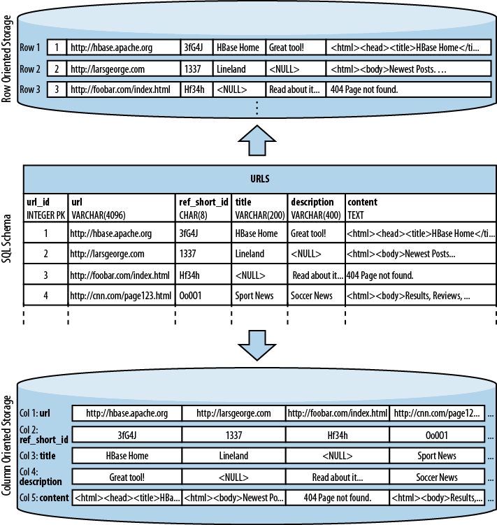
Consider the HBase URL Shortener, Hush, which allows us to map long URLs to short URLs. The entity relationship diagram (ERD) can be seen in Figure 1-2. The full SQL schema can be found in Appendix E.[21]
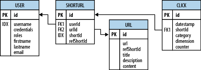
The shortened URL, stored in the shorturl table, can then be given to others
that subsequently click on it to open the linked full URL. Each click is
tracked, recording the number of times it was used, and, for example,
the country the click came from. This is stored in the click table, which aggregates the usage on a
daily basis, similar to a counter.
Users, stored in the user table, can sign up with Hush to create
their own list of shortened URLs, which can be edited to add a
description. This links the user and
shorturl tables with a foreign key
relationship.
The system also downloads the linked page in
the background, and extracts, for instance, the TITLE tag from the HTML, if present. The
entire page is saved for later processing with asynchronous batch jobs,
for analysis purposes. This is represented by the url table.
Every linked page is only stored once, but
since many users may link to the same long URL, yet want to maintain
their own details, such as the usage statistics, a separate entry in the
shorturl is created. This links the
url, shorturl, and click tables.
This also allows you to aggregate statistics
to the original short ID, refShortId,
so that you can see the overall usage of any short URL to map to the
same long URL. The shortId and
refShortId are the hashed IDs
assigned uniquely to each shortened URL. For example, in
http://hush.li/a23eg
Figure 1-3 shows how the same schema could be represented in HBase.
Every shortened URL is stored in a separate table, shorturl, which also contains the usage
statistics, storing various time ranges in separate column families,
with distinct time-to-live settings. The columns form the actual
counters, and their name is a combination of the date, plus an optional
dimensional postfix—for example, the country code.
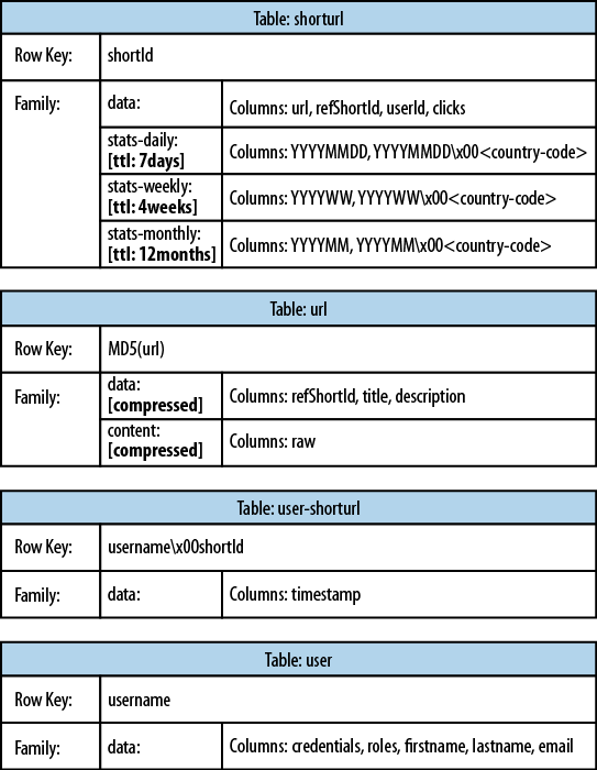
The downloaded page, and the extracted
details, are stored in the url table.
This table uses compression to minimize the storage requirements,
because the pages are mostly HTML, which is inherently verbose and
contains a lot of text.
The user-shorturl table acts as a lookup so that
you can quickly find all short IDs for a given user. This is used on the
user’s home page, once she has logged in. The user table stores the actual user
details.
We still have the same number of tables, but
their meaning has changed: the clicks
table has been absorbed by the shorturl table, while the statistics columns
use the date as their key, formatted as YYYYMMDD—for instance,
20110502—so that they can be accessed sequentially.
The additional user-shorturl table is
replacing the foreign key relationship, making user-related lookups
faster.
There are various approaches to converting one-to-one, one-to-many, and many-to-many relationships to fit the underlying architecture of HBase. You could implement even this simple example in different ways. You need to understand the full potential of HBase storage design to make an educated decision regarding which approach to take.
The support for sparse, wide tables and
column-oriented design often eliminates the need to normalize data and,
in the process, the costly JOIN
operations needed to aggregate the
data at query time. Use of intelligent keys gives you fine-grained
control over how—and where—data is stored. Partial key lookups are
possible, and when combined with compound keys, they have the same
properties as leading, left-edge indexes. Designing the schemas properly
enables you to grow the data from 10 entries to 10 million entries,
while still retaining the same write and read performance.
Building Blocks
This section provides you with an overview of the architecture behind HBase. After giving you some background information on its lineage, the section will introduce the general concepts of the data model and the available storage API, and presents a high-level overview on implementation.
Backdrop
In 2003, Google published a paper titled “The Google File System”. This scalable distributed file system, abbreviated as GFS, uses a cluster of commodity hardware to store huge amounts of data. The filesystem handled data replication between nodes so that losing a storage server would have no effect on data availability. It was also optimized for streaming reads so that data could be read for processing later on.
Shortly afterward, another paper by Google was published, titled “MapReduce: Simplified Data Processing on Large Clusters”. MapReduce was the missing piece to the GFS architecture, as it made use of the vast number of CPUs each commodity server in the GFS cluster provides. MapReduce plus GFS forms the backbone for processing massive amounts of data, including the entire search index Google owns.
What is missing, though, is the ability to access data randomly and in close to real-time (meaning good enough to drive a web service, for example). Another drawback of the GFS design is that it is good with a few very, very large files, but not as good with millions of tiny files, because the data retained in memory by the master node is ultimately bound to the number of files. The more files, the higher the pressure on the memory of the master.
So, Google was trying to find a solution that could drive interactive applications, such as Mail or Analytics, while making use of the same infrastructure and relying on GFS for replication and data availability. The data stored should be composed of much smaller entities, and the system would transparently take care of aggregating the small records into very large storage files and offer some sort of indexing that allows the user to retrieve data with a minimal number of disk seeks. Finally, it should be able to store the entire web crawl and work with MapReduce to build the entire search index in a timely manner.
Being aware of the shortcomings of RDBMSes at scale (see Seek Versus Transfer for a discussion of one fundamental issue), the engineers approached this problem differently: forfeit relational features and use a simple API that has basic create, read, update, and delete (or CRUD) operations, plus a scan function to iterate over larger key ranges or entire tables. The culmination of these efforts was published in 2006 in a paper titled “Bigtable: A Distributed Storage System for Structured Data”, two excerpts from which follow:
Bigtable is a distributed storage system for managing structured data that is designed to scale to a very large size: petabytes of data across thousands of commodity servers.
…a sparse, distributed, persistent multi-dimensional sorted map.
It is highly recommended that everyone interested in HBase read that paper. It describes a lot of reasoning behind the design of Bigtable and, ultimately, HBase. We will, however, go through the basic concepts, since they apply directly to the rest of this book.
HBase is implementing the Bigtable storage architecture very faithfully so that we can explain everything using HBase. Appendix F provides an overview of where the two systems differ.
Tables, Rows, Columns, and Cells
First, a quick summary: the most basic unit is a column. One or more columns form a row that is addressed uniquely by a row key. A number of rows, in turn, form a table, and there can be many of them. Each column may have multiple versions, with each distinct value contained in a separate cell.
This sounds like a reasonable description for a typical database, but with the extra dimension of allowing multiple versions of each cells. But obviously there is a bit more to it.
All rows are always sorted lexicographically by their row key. Example 1-1 shows how this will look when adding a few rows with different keys.
hbase(main):001:0> scan 'table1'
ROW                          COLUMN+CELL
row-1                         column=cf1:, timestamp=1297073325971 ...
row-10                        column=cf1:, timestamp=1297073337383 ...
row-11                        column=cf1:, timestamp=1297073340493 ...
row-2                         column=cf1:, timestamp=1297073329851 ...
row-22                        column=cf1:, timestamp=1297073344482 ...
row-3                         column=cf1:, timestamp=1297073333504 ...
row-abc                       column=cf1:, timestamp=1297073349875 ...
7 row(s) in 0.1100 seconds
Note how the numbering is not in sequence as
you may have expected it. You may have to pad keys to get a proper
sorting order. In lexicographical sorting, each key is compared on a
binary level, byte by byte, from left to right. Since row-1... is less than row-2..., no matter what follows, it is sorted
first.
Having the row keys always sorted can give you something like a primary key index known from RDBMSes. It is also always unique, that is, you can have each row key only once, or you are updating the same row. While the original Bigtable paper only considers a single index, HBase adds support for secondary indexes (see Secondary Indexes). The row keys can be any arbitrary array of bytes and are not necessarily human-readable.
Rows are composed of columns, and those, in turn, are grouped into column families. This helps in building semantical or topical boundaries between the data, and also in applying certain features to them—for example, compression—or denoting them to stay in-memory. All columns in a column family are stored together in the same low-level storage file, called an HFile.
Column families need to be defined when the table is created and should not be changed too often, nor should there be too many of them. There are a few known shortcomings in the current implementation that force the count to be limited to the low tens, but in practice it is often a much smaller number (see Chapter 9 for details). The name of the column family must be composed of printable characters, a notable difference from all other names or values.
Columns are often referenced as
family:qualifier with the qualifier being any arbitrary array of
bytes.[22] As opposed to the limit on column families, there is no
such thing for the number of columns: you could have millions of columns
in a particular column family. There is also no type nor length boundary
on the column values.
Figure 1-4 helps to visualize how different rows are in a normal database as opposed to the column-oriented design of HBase. You should think about rows and columns not being arranged like the classic spreadsheet model, but rather use a tag metaphor, that is, information is available under a specific tag.
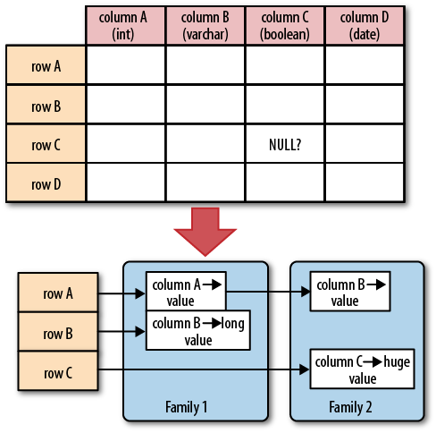
Note
The "NULL?" in Figure 1-4 indicates that, for a database with a
fixed schema, you have to store NULLs where there is no value, but for
HBase’s storage architectures, you simply omit the whole column; in
other words, NULLs are free of any
cost: they do not occupy any storage space.
All rows and columns are defined in the context of a table, adding a few more concepts across all included column families, which we will discuss shortly.
Every column value, or cell, either is timestamped implicitly by the system or can be set explicitly by the user. This can be used, for example, to save multiple versions of a value as it changes over time. Different versions of a cell are stored in decreasing timestamp order, allowing you to read the newest value first. This is an optimization aimed at read patterns that favor more current values over historical ones.
The user can specify how many versions of a value should be kept. In addition, there is support for predicate deletions (see Log-Structured Merge-Trees for the concepts behind them) allowing you to keep, for example, only values written in the past week. The values (or cells) are also just uninterpreted arrays of bytes, that the client needs to know how to handle.
If you recall from the quote earlier, the Bigtable model, as implemented by HBase, is a sparse, distributed, persistent, multidimensional map, which is indexed by row key, column key, and a timestamp. Putting this together, we can express the access to data like so:
(Table, RowKey, Family, Column, Timestamp) → Value
In a more programming language style, this may be expressed as:
SortedMap<
    RowKey, List<
        SortedMap<
            Column, List<
                Value, Timestamp
            >
        >
    >
>SortedMap<RowKey, List<SortedMap<Column, List<Value, Timestamp>>>>
The first SortedMap is the table, containing a List of column families. The families contain
another SortedMap, which represents
the columns, and their associated values. These values are in the final
List that holds the value and the
timestamp it was set.
An interesting feature of the model is that cells may exist in multiple versions, and different columns have been written at different times. The API, by default, provides you with a coherent view of all columns wherein it automatically picks the most current value of each cell. Figure 1-5 shows a piece of one specific row in an example table.
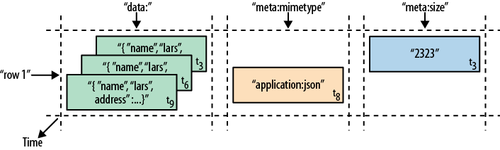
The diagram visualizes the time component
using tn as
the timestamp when the cell was written. The ascending index shows that
the values have been added at different times. Figure 1-6 is another way to look at the data, this time
in a more spreadsheet-like layout wherein the timestamp was added to its
own column.
Although they have been added at different
times and exist in multiple versions, you would still see the row as the
combination of all columns and their most current versions—in other words, the highest
tn from each
column. There is a way to ask for values at (or before) a specific
timestamp, or more than one version at a time, which we will see a
little bit later in Chapter 3.
Access to row data is atomic and includes any number of columns being read or written to. There is no further guarantee or transactional feature that spans multiple rows or across tables. The atomic access is also a contributing factor to this architecture being strictly consistent, as each concurrent reader and writer can make safe assumptions about the state of a row.
Using multiversioning and timestamping can help with application layer consistency issues as well.
Auto-Sharding
The basic unit of scalability and load balancing in HBase is called a region. Regions are essentially contiguous ranges of rows stored together. They are dynamically split by the system when they become too large. Alternatively, they may also be merged to reduce their number and required storage files.[23]
Note
The HBase regions are equivalent to range partitions as used in database sharding. They can be spread across many physical servers, thus distributing the load, and therefore providing scalability.
Initially there is only one region for a table, and as you start adding data to it, the system is monitoring it to ensure that you do not exceed a configured maximum size. If you exceed the limit, the region is split into two at the middle key—the row key in the middle of the region—creating two roughly equal halves (more details in Chapter 8).
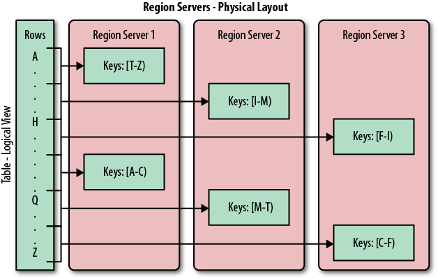
Each region is served by exactly one region server, and each of these servers can serve many regions at any time. Figure 1-7 shows how the logical view of a table is actually a set of regions hosted by many region servers.
Note
The Bigtable paper notes that the aim is to keep the region count between 10 and 1,000 per server and each at roughly 100 MB to 200 MB in size. This refers to the hardware in use in 2006 (and earlier). For HBase and modern hardware, the number would be more like 10 to 1,000 regions per server, but each between 1 GB and 2 GB in size.
But, while the numbers have increased, the basic principle is the same: the number of regions per server, and their respective sizes, depend on what can be handled sufficiently by a single server.
Splitting and serving regions can be thought of as autosharding, as offered by other systems. The regions allow for fast recovery when a server fails, and fine-grained load balancing since they can be moved between servers when the load of the server currently serving the region is under pressure, or if that server becomes unavailable because of a failure or because it is being decommissioned.
Splitting is also very fast—close to instantaneous—because the split regions simply read from the original storage files until a compaction rewrites them into separate ones asynchronously. This is explained in detail in Chapter 8.
Storage API
Bigtable does not support a full relational data model; instead, it provides clients with a simple data model that supports dynamic control over data layout and format [...]
The API offers operations to create and delete tables and column families. In addition, it has functions to change the table and column family metadata, such as compression or block sizes. Furthermore, there are the usual operations for clients to create or delete values as well as retrieving them with a given row key.
A scan API allows you to efficiently iterate over ranges of rows and be able to limit which columns are returned or the number of versions of each cell. You can match columns using filters and select versions using time ranges, specifying start and end times.
On top of this basic functionality are more advanced features. The system has support for single-row transactions, and with this support it implements atomic read-modify-write sequences on data stored under a single row key. Although there are no cross-row or cross-table transactions, the client can batch operations for performance reasons.
Cell values can be interpreted as counters and updated atomically. These counters can be read and modified in one operation so that, despite the distributed nature of the architecture, clients can use this mechanism to implement global, strictly consistent, sequential counters.
There is also the option to run client-supplied code in the address space of the server. The server-side framework to support this is called coprocessors. The code has access to the server local data and can be used to implement lightweight batch jobs, or use expressions to analyze or summarize data based on a variety of operators.
Finally, the system is integrated with the MapReduce framework by supplying wrappers that convert tables into input source and output targets for MapReduce jobs.
Unlike in the RDBMS landscape, there is no domain-specific language, such as SQL, to query data. Access is not done declaratively, but purely imperatively through the client-side API. For HBase, this is mostly Java code, but there are many other choices to access the data from other programming languages.
Implementation
Bigtable [...] allows clients to reason about the locality properties of the data represented in the underlying storage.
The data is stored in store files, called HFiles, which are persistent and ordered immutable maps from keys to values. Internally, the files are sequences of blocks with a block index stored at the end. The index is loaded when the HFile is opened and kept in memory. The default block size is 64 KB but can be configured differently if required. The store files provide an API to access specific values as well as to scan ranges of values given a start and end key.
Note
Implementation is discussed in great detail in Chapter 8. The text here is an introduction only, while the full details are discussed in the referenced chapter(s).
Since every HFile has a block index, lookups can be performed with a single disk seek. First, the block possibly containing the given key is determined by doing a binary search in the in-memory block index, followed by a block read from disk to find the actual key.
The store files are typically saved in the Hadoop Distributed File System (HDFS), which provides a scalable, persistent, replicated storage layer for HBase. It guarantees that data is never lost by writing the changes across a configurable number of physical servers.
When data is updated it is first written to a commit log, called a write-ahead log (WAL) in HBase, and then stored in the in-memory memstore. Once the data in memory has exceeded a given maximum value, it is flushed as an HFile to disk. After the flush, the commit logs can be discarded up to the last unflushed modification. While the system is flushing the memstore to disk, it can continue to serve readers and writers without having to block them. This is achieved by rolling the memstore in memory where the new/empty one is taking the updates, while the old/full one is converted into a file. Note that the data in the memstores is already sorted by keys matching exactly what HFiles represent on disk, so no sorting or other special processing has to be performed.
Note
We can now start to make sense of what
the locality properties are, mentioned
in the Bigtable quote at the beginning of this section. Since all
files contain sorted key/value pairs, ordered by the key, and are
optimized for block operations such as reading these pairs
sequentially, you should specify keys to keep related data together.
Referring back to the webtable example earlier, you may have noted
that the key used is the reversed FQDN (the domain name part of the
URL), such as org.hbase.www. The
reason is to store all pages from hbase.org close to one another, and
reversing the URL puts the most important part of the URL first, that
is, the top-level domain (TLD). Pages under blog.hbase.org would then be sorted with
those from www.hbase.org—or in the
actual key format, org.hbase.blog
sorts next to org.hbase.www.
Because store files are immutable, you cannot simply delete values by removing the key/value pair from them. Instead, a delete marker (also known as a tombstone marker) is written to indicate the fact that the given key has been deleted. During the retrieval process, these delete markers mask out the actual values and hide them from reading clients.
Reading data back involves a merge of what is stored in the memstores, that is, the data that has not been written to disk, and the on-disk store files. Note that the WAL is never used during data retrieval, but solely for recovery purposes when a server has crashed before writing the in-memory data to disk.
Since flushing memstores to disk causes more and more HFiles to be created, HBase has a housekeeping mechanism that merges the files into larger ones using compaction. There are two types of compaction: minor compactions and major compactions. The former reduce the number of storage files by rewriting smaller files into fewer but larger ones, performing an n-way merge. Since all the data is already sorted in each HFile, that merge is fast and bound only by disk I/O performance.
The major compactions rewrite all files within a column family for a region into a single new one. They also have another distinct feature compared to the minor compactions: based on the fact that they scan all key/value pairs, they can drop deleted entries including their deletion marker. Predicate deletes are handled here as well—for example, removing values that have expired according to the configured time-to-live or when there are too many versions.
Note
This architecture is taken from LSM-trees (see Log-Structured Merge-Trees). The only difference is that LSM-trees are storing data in multipage blocks that are arranged in a B-tree-like structure on disk. They are updated, or merged, in a rotating fashion, while in Bigtable the update is more course-grained and the whole memstore is saved as a new store file and not merged right away. You could call HBase’s architecture “Log-Structured Sort-and-Merge-Maps.” The background compactions correspond to the merges in LSM-trees, but are occurring on a store file level instead of the partial tree updates, giving the LSM-trees their name.
There are three major components to HBase: the client library, one master server, and many region servers. The region servers can be added or removed while the system is up and running to accommodate changing workloads. The master is responsible for assigning regions to region servers and uses Apache ZooKeeper, a reliable, highly available, persistent and distributed coordination service, to facilitate that task.
Figure 1-8 shows how the various components of HBase are orchestrated to make use of existing system, like HDFS and ZooKeeper, but also adding its own layers to form a complete platform.
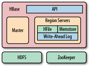
The master server is also responsible for handling load balancing of regions across region servers, to unload busy servers and move regions to less occupied ones. The master is not part of the actual data storage or retrieval path. It negotiates load balancing and maintains the state of the cluster, but never provides any data services to either the region servers or the clients, and is therefore lightly loaded in practice. In addition, it takes care of schema changes and other metadata operations, such as creation of tables and column families.
Region servers are responsible for all read and write requests for all regions they serve, and also split regions that have exceeded the configured region size thresholds. Clients communicate directly with them to handle all data-related operations.
Region Lookups has more details on how clients perform the region lookup.
Summary
Billions of rows * millions of columns * thousands of versions = terabytes or petabytes of storage
We have seen how the Bigtable storage architecture is using many servers to distribute ranges of rows sorted by their key for load-balancing purposes, and can scale to petabytes of data on thousands of machines. The storage format used is ideal for reading adjacent key/value pairs and is optimized for block I/O operations that can saturate disk transfer channels.
Table scans run in linear time and row key lookups or mutations are performed in logarithmic order—or, in extreme cases, even constant order (using Bloom filters). Designing the schema in a way to completely avoid explicit locking, combined with row-level atomicity, gives you the ability to scale your system without any notable effect on read or write performance.
The column-oriented architecture allows for
huge, wide, sparse tables as storing NULLs is free. Because each row is served by
exactly one server, HBase is strongly consistent, and using its
multiversioning can help you to avoid edit conflicts caused by
concurrent decoupled processes or retain a history of changes.
The actual Bigtable has been in production at Google since at least 2005, and it has been in use for a variety of different use cases, from batch-oriented processing to real-time data-serving. The stored data varies from very small (like URLs) to quite large (e.g., web pages and satellite imagery) and yet successfully provides a flexible, high-performance solution for many well-known Google products, such as Google Earth, Google Reader, Google Finance, and Google Analytics.
HBase: The Hadoop Database
Having looked at the Bigtable architecture, we could simply state that HBase is a faithful, open source implementation of Google’s Bigtable. But that would be a bit too simplistic, and there are a few (mostly subtle) differences worth addressing.
History
HBase was created in 2007 at Powerset[25] and was initially part of the contributions in Hadoop. Since then, it has become its own top-level project under the Apache Software Foundation umbrella. It is available under the Apache Software License, version 2.0.
The project home page is http://hbase.apache.org/, where you can find links to the documentation, wiki, and source repository, as well as download sites for the binary and source releases.
Here is a short overview of how HBase has evolved over time:
- November 2006
- February 2007
Initial HBase prototype created as Hadoop contrib[26]
- October 2007
- January 2008
Hadoop becomes an Apache top-level project, HBase becomes subproject
- October 2008
- January 2009
- September 2009
- May 2010
- June 2010
- January 2011
- Mid 2011
HBase 0.92.0 released, tagged as coprocessor and security release
Note
Around May 2010, the developers decided to break with the version numbering that was used to be in lockstep with the Hadoop releases. The rationale was that HBase had a much faster release cycle and was also approaching a version 1.0 level sooner than what was expected from Hadoop.
To that effect, the jump was made quite obvious, going from 0.20.x to 0.89.x. In addition, a decision was made to title 0.89.x the early access version for developers and bleeding-edge integrators. Version 0.89 was eventually released as 0.90 for everyone as the next stable release.
Nomenclature
One of the biggest differences between HBase and Bigtable concerns naming, as you can see in Table 1-1, which lists the various terms and what they correspond to in each system.
| HBase | Bigtable |
| Region | Tablet |
| RegionServer | Tablet server |
| Flush | Minor compaction |
| Minor compaction | Merging compaction |
| Major compaction | Major compaction |
| Write-ahead log | Commit log |
| HDFS | GFS |
| Hadoop MapReduce | MapReduce |
| MemStore | memtable |
| HFile | SSTable |
| ZooKeeper | Chubby |
More differences are described in Appendix F.
Summary
Let us now circle back to Dimensions, and how dimensions can be used to classify HBase. HBase is a distributed, persistent, strictly consistent storage system with near-optimal write—in terms of I/O channel saturation—and excellent read performance, and it makes efficient use of disk space by supporting pluggable compression algorithms that can be selected based on the nature of the data in specific column families.
HBase extends the Bigtable model, which only considers a single index, similar to a primary key in the RDBMS world, offering the server-side hooks to implement flexible secondary index solutions. In addition, it provides push-down predicates, that is, filters, reducing data transferred over the network.
There is no declarative query language as part of the core implementation, and it has limited support for transactions. Row atomicity and read-modify-write operations make up for this in practice, as they cover most use cases and remove the wait or deadlock-related pauses experienced with other systems.
HBase handles shifting load and failures gracefully and transparently to the clients. Scalability is built in, and clusters can be grown or shrunk while the system is in production. Changing the cluster does not involve any complicated rebalancing or resharding procedure, but is completely automated.
[5] See, for example, “‘One Size Fits All’: An Idea Whose Time Has Come and Gone” (http://www.cs.brown.edu/~ugur/fits_all.pdf) by Michael Stonebraker and Uğur Çetintemel.
[6] Information can be found on the project’s website. Please also see the excellent Hadoop: The Definitive Guide (Second Edition) by Tom White (O’Reilly) for everything you want to know about Hadoop.
[7] The quotes are from a presentation titled “Rethinking EDW in the Era of Expansive Information Management” by Dr. Ralph Kimball, of the Kimball Group, available at http://www.informatica.com/campaigns/rethink_edw_kimball.pdf. It discusses the changing needs of an evolving enterprise data warehouse market.
[8] Edgar F. Codd defined 13 rules (numbered from 0 to 12), which define what is required from a database management system (DBMS) to be considered relational. While HBase does fulfill the more generic rules, it fails on others, most importantly, on rule 5: the comprehensive data sublanguage rule, defining the support for at least one relational language. See Codd’s 12 rules on Wikipedia.
[10] See this blog post, as well as this one, by the Facebook engineering team. Wall messages count for 15 billion and chat for 120 billion, totaling 135 billion messages a month. Then they also add SMS and others to create an even larger number.
[11] Facebook uses Haystack, which provides an optimized storage infrastructure for large binary objects, such as photos.
[12] See this presentation, given by Facebook employee and HBase committer, Nicolas Spiegelberg.
[13] Short for Linux, Apache, MySQL, and PHP (or Perl and Python).
[14] Short for Atomicity, Consistency, Isolation, and Durability. See “ACID” on Wikipedia.
[15] Memcached is an in-memory, nonpersistent, nondistributed key/value store. See the Memcached project home page.
[16] See “NoSQL” on Wikipedia.
[17] See Eric Brewer’s original paper on this topic and the follow-up post by Coda Hale, as well as this PDF by Gilbert and Lynch.
[18] See Brewer: “Lessons from giant-scale services.” Internet Computing, IEEE (2001) vol. 5 (4) pp. 46–55 (http://ieeexplore.ieee.org/xpl/freeabs_all.jsp?arnumber=939450).
[20] The term DDI was coined in the paper “Cloud Data Structure Diagramming Techniques and Design Patterns” by D. Salmen et al. (2009).
[21] Note, though, that this is provided purely for demonstration purposes, so the schema is deliberately kept simple.
[22] You will see in Column Families that the qualifier also may be left unset.
[23] Although HBase does not support online region merging, there are tools to do this offline. See Merging Regions.
[24] For more information on Apache ZooKeeper, please refer to the official project website.
[25] Powerset is a company based in San Francisco that was developing a natural language search engine for the Internet. On July 1, 2008, Microsoft acquired Powerset, and subsequent support for HBase development was abandoned.
Get HBase: The Definitive Guide now with the O’Reilly learning platform.
O’Reilly members experience books, live events, courses curated by job role, and more from O’Reilly and nearly 200 top publishers.

