GNU Octave

Time for action – making your first plot

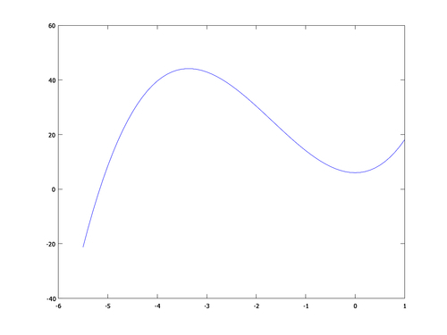
Let us try to plot the polynomial, f, given in Equation (3.1) in the interval x ∈ [–5.5; 1]:

octave:59> x = [-5.5:0.1:1]; f = polyval(c,x);

octave:60> plot(x, f)

You should now see a plot looking somewhat like the one below:

What just happened?

The first input argument to plot is the x variable which is used as the x axis values. The second is f and is used as the y axis values. Note that these two variables must have the same length. If they do not, Octave will issue an error. You can also call plot with a single input argument. In this case, the input variable is plotted against its indices.

When we plot ...