Chapter 1. Why Kudu?
Why Does Kudu Matter?
As big data platforms continue to innovate and evolve, whether on-premises or in the cloud, itâs no surprise that many are feeling some fatigue at the pace of new open source big data project releases. After working with Kudu for the past year with large companies and real-world use cases, weâre more convinced than ever that Kudu matters and that itâs very much worthwhile to add yet another project to the open source big data world.
Our reasoning boils down to three essential points:
-
Big data is still too difficultâas the audience and appetite for data grows, Hadoop and big data platforms are still too difficult, and much of this complexity is driven from limitations in storage. At our office, long-winded architecture discussions are now being cut short with the common refrain, âJust use Kudu and be done with it.â
-
New use cases need Kuduâthe use cases Hadoop is being called upon to serve are changingâthis includes an increasing focus on machine-generated data and real-time analytics. To demonstrate this complexity, we walk through some architectures for real-time analytics using existing big data storage technologies and discuss how Kudu simplifies these architectures.
-
The hardware landscape is changingâmany of the fundamental assumptions about hardware upon which Hadoop was built are changing. There are fresh opportunities to create a storage manager with improved performance and workload flexibility.
In this chapter we discuss the aforementioned motivations in detail. If youâre already familiar with the motivation for Kudu, you can skip to the latter part of this chapter where we discuss some of Kuduâs goals and how Kudu compares to other big data storage systems. We finish up by summarizing why the world needs another big data storage system.
Simplicity Drives Adoption
Distributed systems used to be expensive and difficult. We worked for a large media and information provider in the mid-2000s building a platform for the ingest, processing, search, storage, and retrieval of hundreds of terabytes of online content. Building such a platform was a gargantuan effort involving hundreds of engineers and teams dedicated to building different parts of the platform. We had separate teams dedicated to distributed systems for ingest, storage, search, content retrieval, and so on. To scale our platform, we sharded our relational stores, search indexes, and storage systems and then built elaborate metadata systems on top in order to keep everything sorted out. The platform was built on expensive proprietary technologies that acted as a barrier to ward off smaller competing companies wanting to do the same thing.
Around the same time, Doug Cutting and Mike Carafella were building Apache Hadoop. Thanks to their work and the work of the entire Hadoop ecosystem community, building scale-out infrastructure no longer requires many millions of dollars and huge teams of specialized distributed systems engineers. One of Hadoopâs first advancements was that a software engineer with very modest knowledge of distributed systems had access to scale-out data platforms. It made distributed computing for the software engineer easier.
Although the software engineers rejoiced, that was just a slice of the total population of people wanting access to big data. Hence, the church of big data continued to grow and diversify. Starting with Hive, and then Impala, and then all the other SQL-on-Hadoop engines, analysts and SQL engineers with no programming background have been able to process and analyze their data at scale using Hadoop. By providing a familiar interface, SQL has allowed a huge group of users waiting on the doorstep of Hadoop to be let in. SQL-on-Hadoop mattered because it made data processing and analysis easier and faster versus a programming language. Thatâs not to say that SQL made Hadoop âeasy.â Ask anyone coming from the relational database management system (RDBMS) world and they will tell you that even though SQL certainly made Hadoop more usable, there are plenty of gaps and caveats to watch out for. In addition, especially in the early days, engineers and analysts needed to decide which specific engine or format best fit their particular use case. We talk about the specific challenges later in this chapter, but for now, letâs say that SQL-on-Hadoop made distributed computing easy for the SQL-savvy data engineer.
Note
At the time of this writing, Hive Kudu support is still pending in HIVE-12971. However, itâs still possible to create Hive tables, which Impala accesses.
More users want in on this scalable goodness. With the rise of machine learning and data science, big data platforms are now serving statisticians, mathematicians, and a broader audience of data analysts. Productivity for these users is driven by fast iteration and performance. The effectiveness of the data scientistâs model is often driven by data volume, making Hadoop an obvious choice. These users are familiar with SQL but are not âengineersâ and therefore not interested in dealing with some of Hadoopâs nuances. They expect even better usability, simplicity, and performance.
In addition, traditional enterprise business intelligence and analytics systems people also want in on the Hadoop action, leading to even more demand for performant and mature SQL systems.
Hadoop democratized big data, both technically and econimically, and made it possible for a programmer or software engineer with little knowledge of the intricacies of distributed systems to ingest, store, process, and serve huge amounts of data. Over time, Hadoop has evolved further and can now serve an even broader audience of users. As a result, weâve all been witness to a fairly obvious fact: the easier a data platform is to use, the more adoption it will gain, the more users it can serve, and the more value it can provide. This has certainly been true of Hadoop over the past 10 years. As Hadoop became simpler and easier to use, weâve seen increased adoption and value (Figure 1-1).
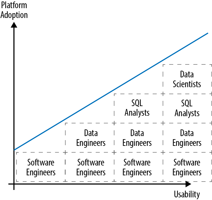
Figure 1-1. Hadoop adoption and simplicity
Kuduâs simplicity grows Hadoopâs âaddressable market.â It does this by providing functionality and a data model closer to what youâd see in an RDBMS. Kudu provides a relational-like table construct for storing data and allows users to insert, update, and delete data, in much the same way that you can with a relational database. This model is familiar to just about everyone who interacts with dataâsoftware engineers, analysts, Extract, Transfer, and Load (ETL) developers, data scientists, statisticians, and so on. In addition, it also aligns with the use cases that Hadoop is being asked to solve today.
New Use Cases
Hadoop is being stretched in terms of the use cases itâs being expected to solve. These use cases are driven by the combined force of several factors. One is the macro-trends of data, like the rise of real-time analytics and the Internet of Things (IoT). These workloads are complex to design properly and can be a brick wall for even experienced Hadoop developers. Another factor is the changing user audience of the platform, as discussed in the previous section. With new users come new use cases and new ways to use the platform. Another factor is increasing expectations of end users of data. Five to ten years ago, batch was okay. After all, we couldnât even process this much data before! But today, being able to scalably store and process data is table stakes; users expect real-time results and speedy performance for a variety of workloads.
Letâs look at some of these use cases and the demands they place on storage.
IoT
By 2020, there are projected to be 20 to 30 billion connected devices in the world. These devices come in every shape and form you can imagine. There are massive âconnected cargo and passenger shipsâ instrumented with sensors monitoring everything from fuel consumption to engines and location. There are now connected cars, connected mining equipment, and connected refrigerators. Implanted medical devices responsible for delivering life-saving therapies like pacing, defibrillation, and neuro-stimulation are now able to emit data that can be used to recognize when a patient is having a medical episode or when there are issues with a device that needs maintenance or replacement.
Billions of connected devices creates an obvious scale problem and makes Hadoop a good choice, but the precise architectural solution is less obvious than you might at first think. Suppose that we have a connected medical device and we want to analyze data from that device. Letâs begin with a simple set of requirements: we want to be able to stream events from connected devices into a storage layer, whatever that might be, and then be able to query the data in just a couple ways. First, we want to be able to see whatâs happening with the device right now. For example, after rolling out a software update to our device, we want to be able look at up-to-the-second signals coming off the device to understand if our update is having the desired effect or encountering any issues. The other access pattern is analytics; we have data analysts who are looking for trends in data to gain new insights to understand and report on device performance, studying, for example, things like battery usage and optimization.
To serve these basic access patterns (Figure 1-2), the storage layer needs the following capabilities:
- Row-by-row inserts
-
When the application server or gateway device receives an event, it needs to be able to save that event to storage, making it immediately available for readers.
- Low-latency random reads
-
After deploying an update to some devices, it needs to analyze the performance of a subset of devices and time. This means being able to efficiently look up a small range of rows.
- Fast analytical scans
-
To serve reporting and ad hoc analytics needs, we need to be able to scan large volumes of data efficiently from storage.
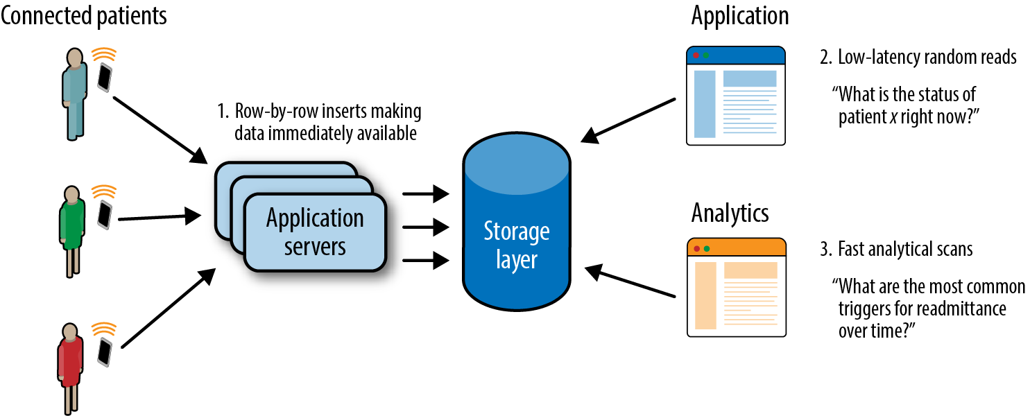
Figure 1-2. IoT access patterns
Current Approaches to Real-Time Analytics
Letâs take a look at a simple example of whatâs required to successfully implement a real-time streaming analytics use case without Kudu.
In this example, we have a data source producing continuous streams of events (Figure 1-3). We need to store these events in near real time, as our users require these events to be made available to them, because the value of this data is highest when itâs first created. The architecture consists of a producer that takes events from the source and then saves them to some yet-to-be-determined storage layer so that the events can be analyzed by business users via SQL, and data scientists and developers using Spark. The concept of the producer is generic; it could be a Flume agent, SparkStreaming job, or a standalone application.
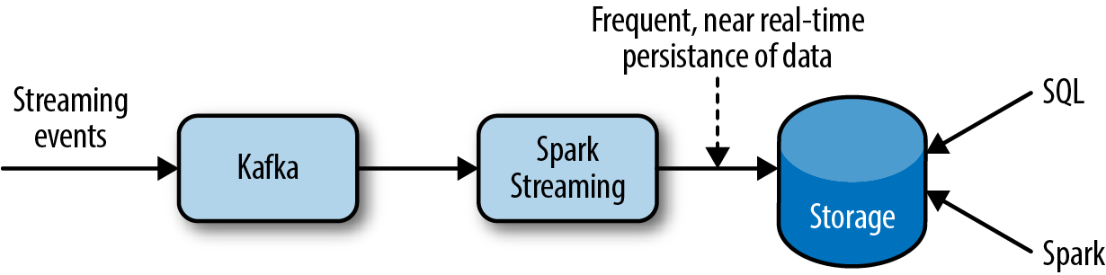
Figure 1-3. Simple real-time analytics flow
Choosing a storage engine for this use case is a surprisingly thorny decision. Letâs take a look at our options using traditional Hadoop storage engines.
Iteration 1: Hadoop Distributed File System
In our first iteration, weâre going to try to keep things simple and save our data in Hadoop Distributed File System (HDFS) as Avro files. While weâre picking on HDFS in this example, these same principles apply when using other storage layers like Amazon Web Services Simple Storage Service (Amazon S3). Avro is a row-based data format. Row-based formats work well with streaming systems because large numbers of rows need to be buffered in memory when writing columnar formats such as Parquet. We create a Hive table, partitioned by date, and from our producer, write microbatches of data as Avro files in HDFS. Because users want access to data soon after creation, the producer is frequently writing new files to HDFS. For example, if our producer were a Spark Streaming application running a micro-batch every 10 seconds, the application would also save a new batch every 10 seconds in order to make the data available to consumers.
We deploy our new system to the production cluster. The high-level data flow now looks like Figure 1-4.
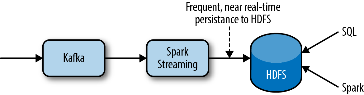
Figure 1-4. Real-time data flow using HDFS
A couple days after deploying the application, the tickets begin flowing. The Operations Team is receiving user reports that performance is slow and their jobs wonât complete. After looking into some of the jobs, we see that our HDFS directory has tens of thousands of tiny files. As it turns out, each of these tiny files ends up requiring HDFS to do a disk seek and destroys the performance of Spark jobs and Impala queries. Unfortunately, the only way to solve this issue is by reducing the number of small files, which is what we do next.
Iteration 2: HDFS + Compactions
After some googling, we find out this is a problem with a well-known solution: adding an HDFS compaction process. The previously mentioned parts of the architecture remain mostly in place; however, because the ingestion process is rapidly creating small files, there is a new offline compaction process. The compaction process takes the many small files and rewrites them into a smaller number of large files. Although the solution seems easy enough, there are a number of complicating factors. For example, the compaction process will run over a partition after itâs no longer active. That compaction process canât overwrite results into that same partition or youâll momentarily lose data and active queries can fail. You could write the result into a separate location and then switch them out using HDFS commands, but even then, two HDFS commands are required and consistency cannot be achieved.
The complications donât stop there. The final HDFS-based solution ends up requiring two separate âlandingâ directories in HDFS: an active version and a passive version, and a âbaseâ directory for compacted data. The architecture now looks like Figure 1-5 (courtesy of the Cloudera Engineering Blog).
This architecture contains multiple HDFS directories, multiple Hive/Impala tables, and several views. Developers must create orchestration to switch writers between the two active/passive landing directories, use the compaction process to move data from âlandingâ to âbaseâ tables, modify the tables and metadata with the new compacted partitions, clean up the old data, and utilize several view modifications to ensure readers are able to see consistent data.
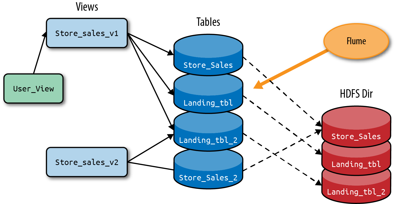
Figure 1-5. Real-time data flow using HDFS with compactions
Even though youâve created an architecture capable of handling large-scale data with lower latency, the solution still has many compromises. For one, the solution is still only pseudo âreal time.â This is because there are still small files, just fewer of them. The more frequently data is written to HDFS, the greater the number of small files, and the efficiency of processing jobs plummets, leading to lower cluster efficiency and job performance. As a result, you might write results to disk only once per minute, so calling this architecture âreal timeâ requires a broad definition of the term. In addition, because HDFS has no notion of a primary key and many stream processing systems have the potential to produce duplicates (i.e., at-least-once versus at-most-once semantics), we need a mechanism that we can use for de-duplication. The result is that our compaction process and table views need to also do de-duplication. Finally, if we have late arriving data, it will not fall within the current dayâs compaction and will result in more small files.
Iteration 3: HBase + HDFS
The complexity and shortcomings mentioned in the previous examples come mostly as a result of trying to get HDFS to do things for which it wasnât optimized or designed. There is yet another and perhaps better-known option in which instead of trying to optimize a single storage layer for nonoptimal performance and usage characteristics, we can marry two storage layers based on their respective strengths. This idea is similar to the Lambda architecture in which you have a âspeed layerâ and a âbatch layer.â The speed layer ingests streaming data and provides storage capable of point lookups on recent data, mutability, and crucially, low-latency reads and writes. For clients needing an up-to-the-second view of the data, the speed layer makes this data available. The traditional Hadoop options for the speed layer are HBase or its âbig tableâ cousin Cassandra. HBase and Cassandra thrive in online, real-time, highly concurrent environments; however, their Achillesâ heel is that they do not provide the fast analytical scan performance of HDFS and Parquet. Thus, to enable fast scans and analytics, you must shift data out of speed layer and into the batch layer of HDFS and Parquet.
Data is now being streamed into our speed layer of HBase or Cassandra. When âenoughâ data has accumulated, a flusher process comes along and moves data from the speed layer to the batch layer. Usually this is done after enough data has accumulated in the speed layer to fill an HDFS partition, so the flusher process is responsible for reading data from the speed layer, rewriting it as Parquet, adding a new partition to HDFS, and then alerting Hive and Impala of the new partition. Because data is now stored in two separate storage managers, clients for this data either need to be aware of the data being in two places, or you must add a service layer to stitch the two layers together to abstract users from this detail. In the end, our architecture looks something like that shown in Figure 1-6.
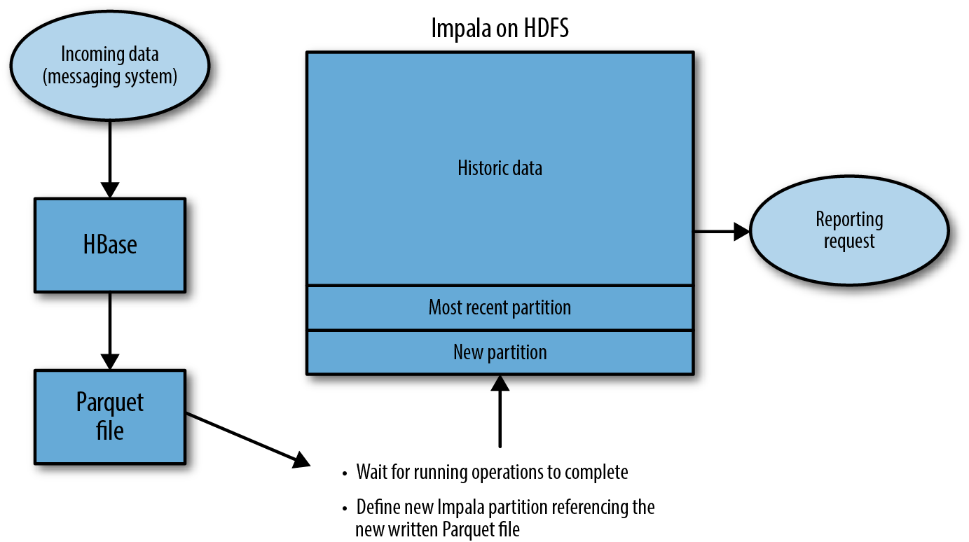
Figure 1-6. Real time data flow using HBase and HDFS
This architecture represents a scale-out solution with the advantages of fresh, up-to-the-second data, mutability, and fast scans. However, it fails when it comes to simplicity of development, operations, and maintenance. Developers are tasked with developing and maintaining code for not only data ingest, but the flusher process to move data out of the speed layer into the batch layer. Operators must now maintain another storage manager, if they arenât already, and must monitor, maintain, and troubleshoot processes for both data ingestion and the process to move data from the speed layer to the batch layer. Lastly, with new and historical data spread between two storage managers, there isnât an easy way for clients to get a unified view from both the speed and batch layers.
These approaches are sophisticated solutions to a seemingly simple problem: scalable, up-to-the-second analytics on rapidly produced data. These solutions arenât easily developed, maintained, or operated. As a result, they tend to be implemented only for use cases in which the value is sure to justify the high level of effort. It is our observation that, due to this complexity, the aforementioned solutions see limited adoption and, in most cases, users settle for a simpler, batch-based solution.
Real-Time Processing
Scalable stream processing is another trend gaining steam in the Hadoop ecosystem. As evidence, you can just look at the number of projects and companies building products in this space. The idea behind stream processing is that rather than saving data to storage and processing the data in batches afterward, events are processed in flight. Unlike batch processing in which there is a defined beginning and end of a batch, in stream processing, the processor is long-lived and operates constantly on small batches of events as they arrive. Stream processing is often used to look at data and make immediate decisions on how to transform, aggregate, filter, or alert on data.
Real-time processing can be useful in model scoring, complex event processing, data enrichment, or many other types of processing. These types of patterns apply in a variety of domains for which the âtime-valueâ of the data is high, meaning that the data is most valuable soon after creation and then diminishes thereafter. Many types of fraud detection, healthcare analytics, and IoT use cases fit this pattern. A major factor limiting adoption of real-time processing is the challenging demands it places on data storage.
Stream processing often requires external context. That context can take many different forms. In some cases, you need historical context and you want to know how the recent data compares to data points in history. In other cases, referential data is required. Fraud detection, for example, relies heavily on both historical and referential data. Historical data will include features like the number of transactions in the past 24 hours or the past week. Referential features might include things like a customerâs account information or the location of an IP address.
Although processing frameworks like Apache Flume, Storm, SparkStreaming, and Flink provide the ability to read and process events in real time, they rely on external systems for storage and access of external context. For example, when using SparkStreaming, you could read micro-batches of events from Kafka every few seconds. If you wanted to be able to save results, read external context, calculate a risk score, and update a patient profile, you now have a diverse set of storage demands:
- Row-by-row inserts
-
As events are being generated, they need to be immediately saved and available for analysis by other tools or processes.
- Low-latency random reads
-
When a streaming engine encounters an event, it might need to look up specific reference information related to that event. For example, if the event represents data from a medical device, specific contextual information about the patient might be needed, such as the name of their clinic or particular information related to their condition.
- Fast analytical scans
-
How does this event relate to history? Being able to run fast analytical scans and SQL in order to gain historical context is often important.
- Updates
-
Contextual information can change. For example, contextual information being fed from Online Transactional Processing (OLTP) applications might populate reference data like contact information, or a patientâs risk score might be updated as new information is computed.
When examining these use cases, youâve surely noticed the theme of having âreal-timeâ capabilities. And you might correctly point out that many organizations are successfully accomplishing the use cases we just mentioned on Hadoop without Kudu. This is true; taken separately, the Hadoop storage layers can handle fast inserts, low-latency random reads, updates, and fast scans. Low-latency reads and writes of your data, yep, got HBase for that. Fast analytics? HDFS can scan your data like nobodyâs businessâwhat else you got? Looking for something simple to use? Sure, we can batch ingest your files into HDFS with one command! The trouble comes when you ask for all those things: row-by-row inserts, random-reads, fast scan, and updatesâall in one. This leads to complex, often difficult to maintain architectures as demonstrated in Figure 1-7.
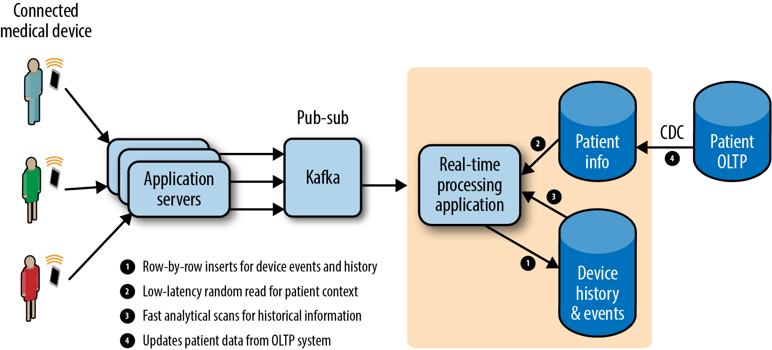
Figure 1-7. Real-time data flow
Handling this diverse list of storage characteristics is possible in many relational databases but immensely difficult using Hadoop and big data. The brutal reality of Hadoop is that these use cases are difficult because the platform forces you to choose storage layers based on a subset of these characterstics.
Hardware Landscape
Hadoop was designed with specific hardware performance and cost considerations in mind. If we go back 15 or so years, when the ideas for Hadoop originated, a reasonably priced server contained some CPU, letâs say 8 or 16 GB of DRAM, and exclusively spinning disks. Hadoop was ingeniously designed to maximize cost and performance, minimizing the use of expensive DRAM and avoiding precious disk seeks to maximize throughput. The steady march of Mooreâs Law has ensured that more bits can fit on our memory chips as well. Commodity servers now have several hundreds of gigabytes of DRAM, tens of terabytes of disk, and increasingly, new types of nonvolatile storage.
This brings us to one of the most dramatic changes happening in hardware today. An average server today is increasingly likely to contain some solid-state, or NAND, storage, which brings new potential. Solid-state drive (SSD) storage brings huge changes in performance characteristics and the removal of many traditional bottlenecks in computing. Specifically, NAND-based storage can handle more I/O, is capable of throughput, and has lower latency seeks versus the traditional hard-disk drive (HDD). Newer trends like three-dimensional NAND strorage are exaggerating these performance changes even further. An L1 cache reference takes about half a nanosecond, DRAM is about 200 nanoseconds, 3D-XPoint (3D NAND from Intel) takes about 7,000 nanoseconds, an SSD drive around 100,000 nanoseconds, and a disk seek is 10 million nanoseconds. To understand the scale of the performance difference between these mediums, suppose that the L1 cache reference is one second. In equivalent terms, a DRAM read would be about six minutes, 3D NAND (3D XPoint, in this case) would be around four hours, an SSD would be a little more than two days, and an HDD seek would be around seven months.
Speed and performance have profound implications on system design. Think about how the speed of transport enabled by automobiles reshaped the worldâs cities and suburbs in the 20th century. With the birth of the car, people were suddenly able to live further away from city centers while still having access to the ammenities and services of a city via automobile. Cities sparawled and suburbs were born. However, with all these fast cars on the road, a new bottleneck arose, and suddenly there was traffic! As a result of all the fast cars, we had to create larger and more efficient roads.
In the context of Hadoop and Kudu, the shift to NAND storage dramatically lowers the computational cost of a disk seek, meaning a storage system can do more of them. If youâre using SSD for storage, you expect to be able to reasonably serve new workloads with random read/write for increased flexibility. SSDs also bring improvements in Input/output operations per second (IOPS) and throughput, so as data is being brought to the CPU more efficiently, this sets up the potential for a new bottleneckâthe CPU. As we look further into the future and these trends are further exaggerated, data platforms should be able to take advantage of improved random I/O performance and should be CPU efficient.
As you might expect, if you purchase one (or one thousand) of these servers, you expect your software to be able to fully utilize its advantages. Practically speaking, this means that if your servers now have hundreds of gigabytes of RAM, you are able to scale your heap to serve more data from memory and see reduced latency.
The hardware landscape continues to evolve and the bottlenecks, cost considerations, and performance of hardware are vastly different today than they were 20 years ago when the ideas behind Hadoop first began. These trends continue to and will continue to change rapidly.
Kuduâs Unique Place in the Big Data Ecosystem
Like other parts of Hadoop, Kudu is designed to be scalable and fault tolerant. Kudu is explicitly a storage layer; therefore, it is not meant to process data and instead relies on the external processing engines of Hadoop, like MapReduce, Spark, or Impala, for that functionality. Although it integrates with many Hadoop components, Kudu can also run as a self-contained, standalone storage engine and does not depend on other frameworks like HDFS or Zookeeper. Kudu stores data in its own columnar format natively in the underlying Linux filesystem and does not utilize HDFS in any way, unlike HBase, for instance.
Kuduâs data model will be familiar to anyone coming from an RDBMS background. Even though Kudu is not a SQL engine itself, its data model is similar to that of a database. Tables are created with a fixed number of typed columns, and a subset of those columns will make up your primary key. As in an RDBMS, the primary key enforces uniqueness for that row. Kudu utilizes a columnar format on disk; this enables efficient encoding and fast scans on a subset of columns. To achieve scale and fault-tolerance, Kudu tables are broken up into horizontal chunks, called tablets, and writes are replicated among tablets using a consensus algorithm, called Raft.
Kuduâs design is fueled by a keen understanding of complex architectures and limitations in present-day Hadoop as well as stark difference developers and architects have to make when choosing a storage engine. Kudu acts as a moderate choice with the goal of having a strong breadth of capabilities and good performance for a variety of workloads. Specifically, Kudu blends low-latency random access, row-by-row inserts, updates, and fast analytical scans into a single storage layer. As discussed, venerable storage engines of HDFS, HBase, and Cassandra have each of these capabilities in isolation; none have all of these capabilities themselves. This difference in workload characteristics between existing Hadoop storage engines is referred to as the analytical gap and is illustrated in Figure 1-8.
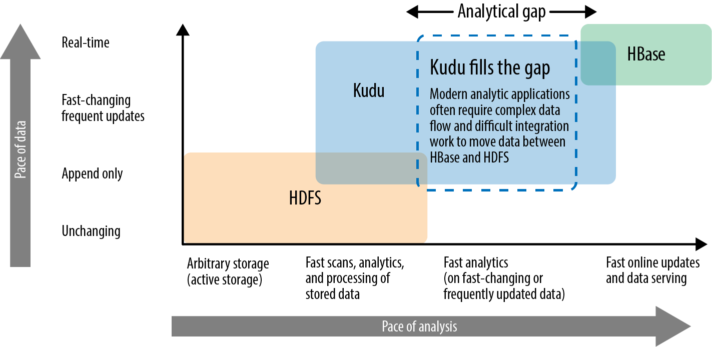
Figure 1-8. Kudu fills the storage gap
HDFS is an append-only filesystem; it performs best with large files for which a processing engine can scan huge amounts of data sequentially. On the other end of the spectrum is Apache HBase or its big table cousins like Cassandra. HBase and Cassandra brought real-time reads and writes and other features needed for online OLTP-like workloads. HBase thrives in online, real-time, highly concurrent environments with mostly random reads and writes or short scans.
Youâll notice in the illustration that Kudu doesnât claim to be faster than HBase or HDFS for any one particular workload. Kudu has high throughput scans and is fast for analytics. Kuduâs goal is to be within two times of HDFS with Parquet or ORCFile for scan performance. Like HBase, Kudu has fast, random reads and writes for point lookups and updates, with the goal of one millisecond read/write latencies on SSD.
If we revisit our earlier real-time analytics use case, this time using Kudu, youâll notice that our architecture is dramatically simpler (Figure 1-9). The first thing to note is that there is a single storage and there are not user-initiated compactions or storage optimization processes. For the operators, they have only one system to monitor and maintain, and they donât need to mess with cron jobs to shuffle data between speed and batch layers, or among Hive partitions. Developers donât need to deal with writing data maintenance code or handle special cases for late arriving data, and updates are handled with ease. For the users, they have immediate access to their real-time and historical data, all in one place.
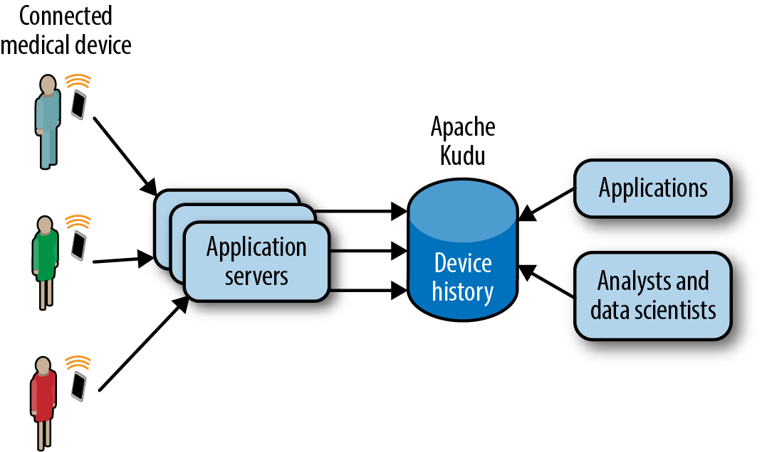
Figure 1-9. Architecture with Kudu
Comparing Kudu with Other Ecosystem Components
Kudu is a new storage system. With the hundreds of databases that have been created over the past 10 years, we personally feel fatigued. Why another storage system? In this section, we continue to answer that question by comparing Kudu against the landscape of traditional ecosystem components.
The easiest comparison is with the SQL engines such as Hive, Impala, and SparkSQL. Kudu doesnât execute SQL queries in whole. There are parts of the SQL query that can be pushed down to the storage layer, such as projection and predicates, which are indeed executed in Kudu. However, a SQL engine has parsers, a planner, and a method for executing the queries. Kudu functions only during query execution and provides input to the planner. Furthermore, Kudu must have projection and predicates pushed down or communicated to it by the SQL engine to participate in the execution of the query and act as more than a simple storage engine.
Now letâs compare Kudu against a traditional relational database. To discuss this, we need to define the types of relational databases. Broadly speaking, there are two kinds of relational databases, Online Transactional Processing (OLTP) and Online Analytical Processing (OLAP) (Figure 1-10). OLTP databases are used for online services on websites, point of sale (PoS), and other applications for which users expect immediate response and strong data integrity. However, typically OLTP databases do not perform well at large scans, which are common in analytical workloads. For example, when servicing a website, an orders page will commonly display all orders for a particular user, e.g., âMy Ordersâ on any online website. However in an analytical context you typically donât care about orders for a particular user, you care about all sales of a given product and often all sales of a particular provider grouped by, for instance, state. OLAP databases perform these types of queries well because they are optimized for scans. Typically, OLAP databases perform poorly at the types of use cases for which OLTP databases are good ; for example, selects of a small number of rows and commonly integrity. You might be surprised that any database would sacrifice on integrity, but OLAP databases are typically loaded in batches, so if anything goes wrong, the entire batch is reloaded without any data loss.
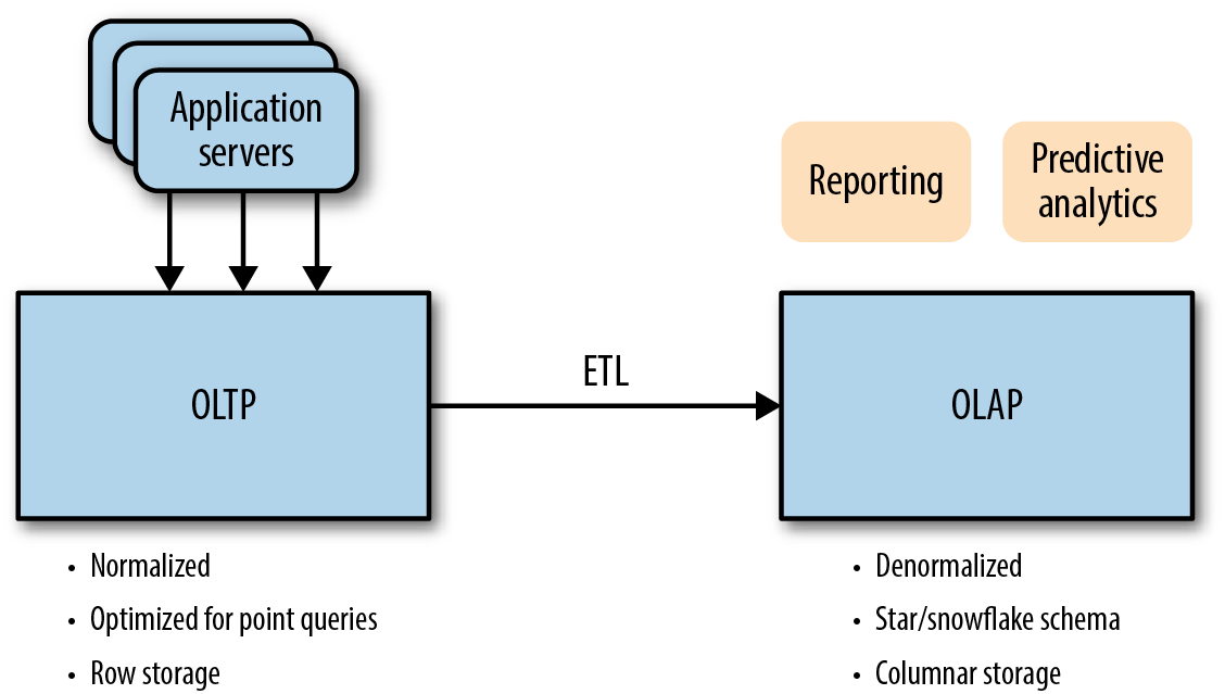
Figure 1-10. OLTP and OLAP
There is another concept we must be aware of before proceeding. Rows of data can be stored in row or column format (see Figures 1-11 and 1-12). Typically, OLTP databases use row format, whereas OLAP databases use columnar. Row formats are great for full-row retreivals and updates. Columnar formats are great for large scans that select a subset of the columns. A typical OLTP query is to get the full row, whereas a typical OLAP query retrieves only part of the row.
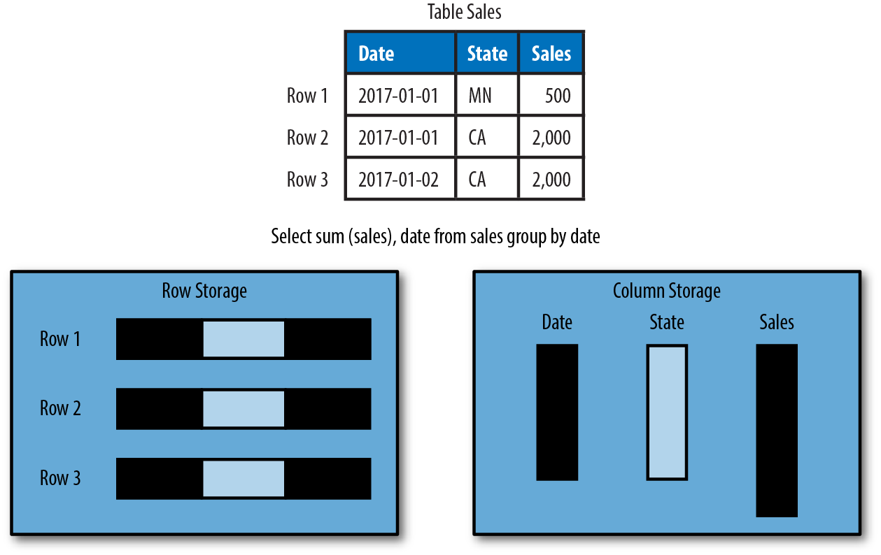
Figure 1-11. Row and column storage, part 1
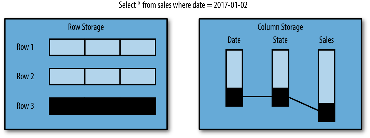
Figure 1-12. Row and column storage, part 2
Not to beat a dead horse, but if you imagine a âMy Ordersâ page on an online store, you will see all relevant information about the order including the billing and shipping addresses along with product name, code, quantity, and price. However, for a query that calculates total sales for a given product by state, the only fields of interest are the product name, quantity, price, and billing state.
Now that we have defined OLTP and OLAP along with row and column format, we can finally compare Kudu versus relational database systems. Today, Kudu is most often thought of as a columnar storage engine for OLAP SQL query engines Hive, Impala, and SparkSQL. However, because rows can be quickly retrieved by primary key and continuously ingested all while the table is being scanned for analytical queries, Kudu has some properties of both OLTP and OLAP systems, putting it in a third category that we discuss later.
There are many, many kinds of relational databases in both the OLTP and OLAP spaces ranging from single process databases such SQLite (OLTP) to shared everything partitioned databases such as Oracle RAC (OLTP/OLAP) to shared nothing partitioned databases such as MySQL Cluster (OLTP) and Vertica (OLAP). Kudu has much in common with relational databases; for example, Kudu tables have a unique primary key, unlike HBase and Cassandra. However, features that are common in relational databases such as common types of transactional support, foreign keys, and nonprimary key indexes are not supported in Kudu. These are all possible and on the roadmap, but not yet implemented.
Kudu plus Impala is most similar to Vertica. Vertica is a postgres variation using storage based on a system called C-Store from which Kudu also takes some heritage. However, there are important differences. First, because the Hadoop ecosystem is not vertically integrated liked traditional databases, we can bring many query engines to the same storage systems. Second, because Kudu implemented a quorum-based storage system, it has stronger durability guarantees. Third, because Hadoop-based query engines schedule work where data resides locally, as opposed to using a shared storage system such as SAN, queries benefit from what is known as data locality. Data locality just means that the âworkâ can read data from a local disk, which typically has less contention than a shared storage device. Some databases like Vertica, which are based on shared-nothing design, can also schedule work âcloseâ to the data. But they can schedule only Vertica queries, close to the data. You can extend them to add new engines and workloads on account of their vertically integrated nature.
Kudu today has some OLAP and OLTP characteristics minus cross-row Atomicity, Consistency, Isolation, Durability (ACID) transactions, putting it in a category known as Hybrid Transactional/Analytic Processing (HTAP). For example, Kudu was built to allow for fast record retrieval by primary key and continuous ingest along with constant analytics. OLAP databases donât often perform well with this mix of use cases. Additionally, Kuduâs durability guarantees are closer to an OLTP database than OLAP. Long term, it can be even stronger with synchronous cross-datacenter replication similar to Google Spanner, an OLTP system. Kudu with its quorum capability has the ability to implement what is known as Fractured Mirrors in which one or two nodes in a quorum use a row format, whereas the third node stores data in a column format. This would allow you to schedule OLTP-style queries on row-format nodes, whereas you can perform OLAP queries on the columnar nodes, mixing both workloads. Lastly, the underlying hardware is changing, which also, given sufficient support, can blur the lines between these two kinds of databases. For example, a big problem when using a columnar database for an OLTP workload is that OLTP workloads often want to retrieve a large subset of a row; in a columnar database that can translate to many disk seeks. However, SSD and persistent memory are mostly eliminating this problem.
Big DataâHDFS, HBase, Cassandra
With all this in mind, how does Kudu compare against other big data storage systems such as HDFS, HBase, and Cassandra? Letâs define at a high level what these other systems do well. HDFS is extremely good when a program is scanning large volumes of data. In short, itâs fantastic at âfull-table scans,â which are extremely common in analytical workloads. HBase and Cassandra are great at random access, reading or modifying data at random. HDFS is poor at random reads, and although it cannot technically perform random writes, you can simulate them through a merge process, which is expensive. HBase and Cassandra, on the other hand, perform extremely poorly relative to HDFS at large scans. Kuduâs goal is to be within two times that of Parquet on HDFS for scans, and similarly close to HBase and Cassandra for random reads. The actual random read goal is one millisecond read/write on SSD.
We go into a little more detail on each system so as to describe why HDFS, HBase, Cassandra, and Kudu perform the way they do. HDFS is a purely distributed filesystem that was designed to perform fast, large scans. After all, the first use case for this design was to build an index of the web in batch. For that use case, and many others, you simply need to be able to scan the entire dataset in a performant manner. HDFS partitions data and spreads it out over a large number of physical disks so that these large scans can utilize many drives in parallel.
HBase and Cassandra are similar to Kudu in that they store data in rows and columns and provide the ability to randomly access the data. However, when it comes to storing data on disk, they store it much differently than Kudu. There are many reasons Kudu is faster at scanning data than these systems, but one of the major reasons is that HBase and Cassandra store data in column families; as such, they are not truly columnar. The net result is twofold: first, data cannot be encoded in columns, which results in extreme compression (as discussed later similar data stored âcloseâ to each other compresses better) and second, one column in the family cannot be scanned without physically reading the other columns.
Another reason Kudu is faster for large scans is that it doesnât perform scan-time merges. Kudu doesnât guarantee that scans return data in exact primary key order (fine for most analytic use cases), and thus we donât need to perform any âmergeâ between different RowSets (chunks of rows). The âmergeâ in HBase happens for two reasons: to provide order, to allow new versions of cells or tombstones to overwrite earlier versions. We donât need the first because we donât guarantee order, and we donât need the second because we use an entirely different delta-tracking design. Rather than storing different versions of each cell, we store base data, and then separate blocks with deltas forward/backward from there. If you have had few recent updates, forward deltas get compacted into REDOs and only backward UNDOs are stored. Then, for a current-time query, we know that we can disregard all backward deltas, meaning that we need to read only the base data.
Reading the base data is very efficient because of its columnar and dense nature. Having schemas means that we donât need to encode column names or value lengths for each cell, and having the deltas segregated means that we donât need to look at timestamps either, resulting in a scan that is nearly as efficient as Parquet.
One particular reason for efficiency relative to HBase is that in avoiding all of these per-cell comparisons, we avoid a lot of CPU branch mispredictions. Each generation of CPUs over the past 10 years has had a deeper pipeline and thus a more expensive branch misprediction cost, and so we get a lot more âbang for the buckâ per CPU cycle.
Conclusion
Kudu is neither appropriate for all situations nor will it completely replace venerable storage engines like HDFS or newer cloud storage like Amazon S3 or Microsoft Azure Data Lake Store. In addition, there are certainly use cases for HBase and Cassandra that Kudu cannot fill today. However, there is a strong wind in the market, and itâs pushing data systems toward even greater scale, toward analytics, toward machine learning, and toward doing all of these things in an operational and real-time wayâthat is to say, production-scale, operational systems run machine learning and analytics to deliver a product or service to an end user. Being able to serve this blend of operational and analytical capabilities is the unique realm of Kudu. As weâve demonstrated in this chapter, there are many ways to build such systems, but without Kudu, your architecture will likely be complex to develop and operate, and your datasets might even be split between different storage engines.
Get Getting Started with Kudu now with the O’Reilly learning platform.
O’Reilly members experience books, live events, courses curated by job role, and more from O’Reilly and nearly 200 top publishers.

