Chapter 4. Beyond Gradient Descent
The Challenges with Gradient Descent
The fundamental ideas behind neural networks have existed for decades, but it wasn’t until recently that neural network-based learning models have become mainstream. Our fascination with neural networks has everything to do with their expressiveness, a quality we’ve unlocked by creating networks with many layers. As we have discussed in previous chapters, deep neural networks are able to crack problems that were previously deemed intractable. Training deep neural networks end to end, however, is fraught with difficult challenges that took many technological innovations to unravel, including massive labeled datasets (ImageNet, CIFAR, etc.), better hardware in the form of GPU acceleration, and several algorithmic discoveries.
For several years, researchers resorted to layer-wise greedy pre-training in order to grapple with the complex error surfaces presented by deep learning models.1 These time-intensive strategies would try to find more accurate initializations for the model’s parameters one layer at a time before using mini-batch gradient descent to converge to the optimal parameter settings. More recently, however, breakthroughs in optimization methods have enabled us to directly train models in an end-to-end fashion.
In this chapter, we will discuss several of these breakthroughs. The next couple of sections will focus primarily on local minima and whether they pose hurdles for successfully training deep models. In subsequent sections, we will further explore the nonconvex error surfaces induced by deep models, why vanilla mini-batch gradient descent falls short, and how modern nonconvex optimizers overcome these pitfalls.
Local Minima in the Error Surfaces of Deep Networks
The primary challenge in optimizing deep learning models is that we are forced to use minimal local information to infer the global structure of the error surface. This is a hard problem because there is usually very little correspondence between local and global structure. Take the following analogy as an example.
Let’s assume you’re an ant on the continental United States. You’re dropped randomly on the map, and your goal is to find the lowest point on this surface. How do you do it? If all you can observe is your immediate surroundings, this seems like an intractable problem. If the surface of the US was bowl shaped (or mathematically speaking, convex) and we were smart about our learning rate, we could use the gradient descent algorithm to eventually find the bottom of the bowl. But the surface of the US is extremely complex, that is to say, is a nonconvex surface, which means that even if we find a valley (a local minimum), we have no idea if it’s the lowest valley on the map (the global minimum). In Chapter 2, we talked about how a mini-batch version of gradient descent can help navigate a troublesome error surface when there are spurious regions of magnitude zero gradients. But as we can see in Figure 4-1, even a stochastic error surface won’t save us from a deep local minimum.
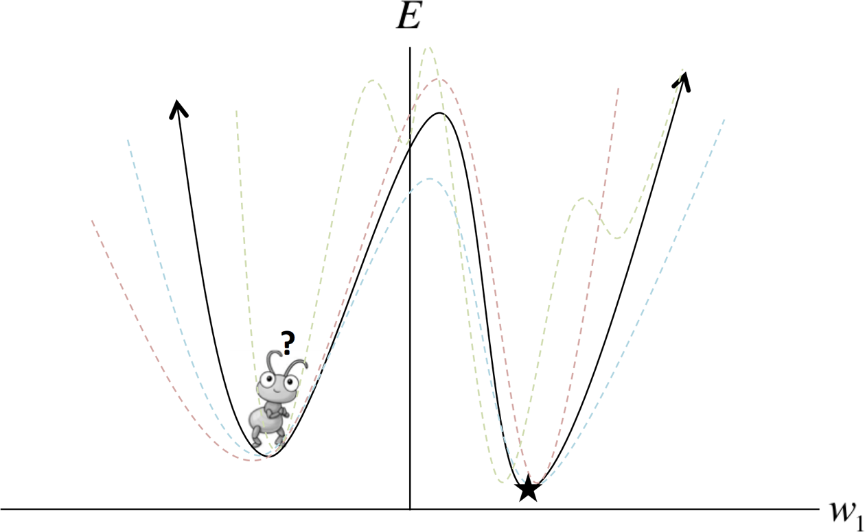
Figure 4-1. Mini-batch gradient descent may aid in escaping shallow local minima, but often fails when dealing with deep local minima, as shown
Now comes the critical question. Theoretically, local minima pose a significant issue. But in practice, how common are local minima in the error surfaces of deep networks? And in which scenarios are they actually problematic for training? In the following two sections, we’ll pick apart common misconceptions about local minima.
Model Identifiability
The first source of local minima is tied to a concept commonly referred to as model identifiability. One observation about deep neural networks is that their error surfaces are guaranteed to have a large—and in some cases, an infinite—number of local minima. There are two major reasons this observation is true.
The first is that within a layer of a fully-connected feed-forward neural network, any rearrangement of neurons will still give you the same final output at the end of the network. We illustrate this using a simple three-neuron layer in Figure 4-2. As a result, within a layer with neurons, there are ways to rearrange parameters. And for a deep network with layers, each with neurons, we have a total of equivalent configurations.
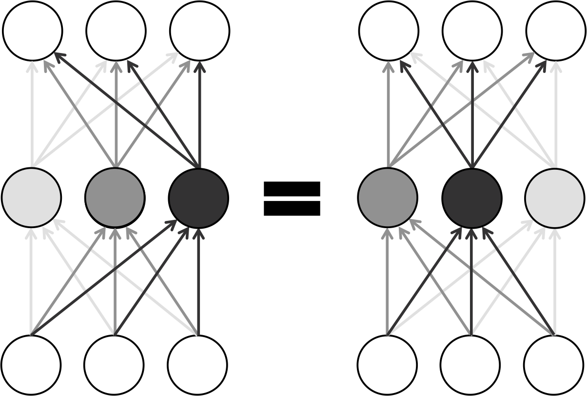
Figure 4-2. Rearranging neurons in a layer of a neural network results in equivalent configurations due to symmetry
In addition to the symmetries of neuron rearrangements, non-identifiability is present in other forms in certain kinds of neural networks. For example, there is an infinite number of equivalent configurations that for an individual ReLU neuron result in equivalent networks. Because an ReLU uses a piecewise linear function, we are free to multiply all of the incoming weights by any nonzero constant while scaling all of the outgoing weights by without changing the behavior of the network. We leave the justification for this statement as an exercise for the active reader.
Ultimately, however, local minima that arise because of the non-identifiability of deep neural networks are not inherently problematic. This is because all nonidentifiable configurations behave in an indistinguishable fashion no matter what input values they are fed. This means they will achieve the same error on the training, validation, and testing datasets. In other words, all of these models will have learned equally from the training data and will have identical behavior during generalization to unseen examples.
Instead, local minima are only problematic when they are spurious. A spurious local minimum corresponds to a configuration of weights in a neural network that incurs a higher error than the configuration at the global minimum. If these kinds of local minima are common, we quickly run into significant problems while using gradient-based optimization methods because we can only take into account local structure.
How Pesky Are Spurious Local Minima in Deep Networks?
For many years, deep learning practitioners blamed all of their troubles in training deep networks on spurious local minima, albeit with little evidence. Today, it remains an open question whether spurious local minima with a high error rate relative to the global minimum are common in practical deep networks. However, many recent studies seem to indicate that most local minima have error rates and generalization characteristics that are very similar to global minima.
One way we might try to naively tackle this problem is by plotting the value of the error function over time as we train a deep neural network. This strategy, however, doesn’t give us enough information about the error surface because it is difficult to tell whether the error surface is “bumpy,” or whether we merely have a difficult time figuring out which direction we should be moving in.
To more effectively analyze this problem, Goodfellow et al. (a team of researchers collaborating between Google and Stanford) published a paper in 2014 that attempted to separate these two potential confounding factors.2 Instead of analyzing the error function over time, they cleverly investigated what happens on the error surface between a randomly initialized parameter vector and a successful final solution by using linear interpolation. So given a randomly initialized parameter vector and stochastic gradient descent (SGD) solution , we aim to compute the error function at every point along the linear interpolation .
In other words, they wanted to investigate whether local minima would hinder our gradient-based search method even if we knew which direction to move in. They showed that for a wide variety of practical networks with different types of neurons, the direct path between a randomly initialized point in the parameter space and a stochastic gradient descent solution isn’t plagued with troublesome local minima.
We can even demonstrate this ourselves using the feed-foward ReLU network we built in Chapter 3. Using a checkpoint file that we saved while training our original feed-forward network, we can re-instantiate the inference and loss components while also maintaining a list of pointers to the variables in the original graph for future use in var_list_opt (where opt stands for the optimal parameter settings):
# mnist data image of shape 28*28=784
x = tf.placeholder("float", [None, 784])
# 0-9 digits recognition => 10 classes
y = tf.placeholder("float", [None, 10])

sess = tf.Session()

with tf.variable_scope("mlp_model") as scope:
    output_opt = inference(x)
    cost_opt = loss(output_opt, y)
    saver = tf.train.Saver()
    scope.reuse_variables()
    var_list_opt = [
        "hidden_1/W",
        "hidden_1/b",
        "hidden_2/W",
        "hidden_2/b",
        "output/W",
        "output/b"
    ]
    var_list_opt = [tf.get_variable(v) for v in var_list_opt]
    saver.restore(sess, "mlp_logs/model-checkpoint-file")
Similarly, we can reuse the component constructors to create a randomly initialized network. Here we store the variables in var_list_rand for the next step of our program:
with tf.variable_scope("mlp_init") as scope:
    output_rand = inference(x)
    cost_rand = loss(output_rand, y)
    scope.reuse_variables()
    var_list_rand = [
        "hidden_1/W",
        "hidden_1/b",
        "hidden_2/W",
        "hidden_2/b",
        "output/W",
        "output/b"
    ]
    var_list_rand = [tf.get_variable(v) for v in var_list_rand]
    init_op = tf.initialize_variables(var_list_rand)
    sess.run(init_op)
With these two networks appropriately initialized, we can now construct the linear interpolation using the mixing parameters alpha and beta:
with tf.variable_scope("mlp_inter") as scope:

    alpha = tf.placeholder("float", [1, 1])
    beta = 1 - alpha

    h1_W_inter = var_list_opt[0] * beta + var_list_rand[0] * alpha
    h1_b_inter = var_list_opt[1] * beta + var_list_rand[1] * alpha
    h2_W_inter = var_list_opt[2] * beta + var_list_rand[2] * alpha
    h2_b_inter = var_list_opt[3] * beta + var_list_rand[3] * alpha
    o_W_inter = var_list_opt[4] * beta + var_list_rand[4] * alpha
    o_b_inter = var_list_opt[5] * beta + var_list_rand[5] * alpha


    h1_inter = tf.nn.relu(tf.matmul(x, h1_W_inter) + h1_b_inter)
    h2_inter = tf.nn.relu(tf.matmul(h1_inter, h2_W_inter) + h2_b_inter)
    o_inter = tf.nn.relu(tf.matmul(h2_inter, o_W_inter) + o_b_inter)


    cost_inter = loss(o_inter, y)
Finally, we can vary the value of alpha to understand how the error surface changes as we traverse the line between the randomly initialized point and the final SGD solution:
import matplotlib.pyplot as plt

summary_writer = tf.train.SummaryWriter("linear_interp_logs/",
                                      graph_def=sess.graph_def)
summary_op = tf.merge_all_summaries()
results = []
for a in np.arange(-2, 2, 0.01):
    feed_dict = {
        x: mnist.test.images,
        y: mnist.test.labels,
        alpha: [[a]],
    }
    cost, summary_str = sess.run([cost_inter, summary_op],
                                 feed_dict=feed_dict)
    summary_writer.add_summary(summary_str, (a + 2)/0.01)
    results.append(cost)


plt.plot(np.arange(-2, 2, 0.01), results, 'ro')
plt.ylabel('Incurred Error')
plt.xlabel('Alpha')
plt.show()
This creates Figure 4-3, which we can inspect ourselves. In fact, if we run this experiment over and over again, we find that there are no truly troublesome local minima that would get us stuck. In other words, it seems that the true struggle of gradient descent isn’t the existence of troublesome local minima, but instead, is that we have a tough time finding the appropriate direction to move in. We’ll return to this thought a little later.
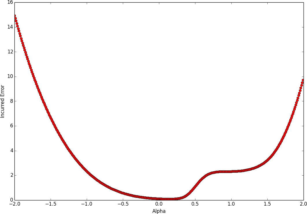
Figure 4-3. The cost function of a three-layer feed-forward network as we linearly interpolate on the line connecting a randomly initialized parameter vector and an SGD solution
Flat Regions in the Error Surface
Although it seems that our analysis is devoid of troublesome local minimum, we do notice a peculiar flat region where the gradient approaches zero when we get to approximately alpha=1. This point is not a local minima, so it is unlikely to get us completely stuck, but it seems like the zero gradient might slow down learning if we are unlucky enough to encounter it.
More generally, given an arbitrary function, a point at which the gradient is the zero vector is called a critical point. Critical points come in various flavors. We’ve already talked about local minima. It’s also not hard to imagine their counterparts, the local maxima, which don’t really pose much of an issue for SGD. But then there are these strange critical points that lie somewhere in-between. These “flat” regions that are potentially pesky but not necessarily deadly are called saddle points. It turns out that as our function has more and more dimensions (i.e., we have more and more parameters in our model), saddle points are exponentially more likely than local minima. Let’s try to intuit why.
For a one-dimensional cost function, a critical point can take one of three forms, as shown in Figure 4-4. Loosely, let’s assume each of these three configurations is equally likely. This means given a random critical point in a random one-dimensional function, it has one-third probability of being a local minimum. This means that if we have a total of critical points, we can expect to have a total of local minima.
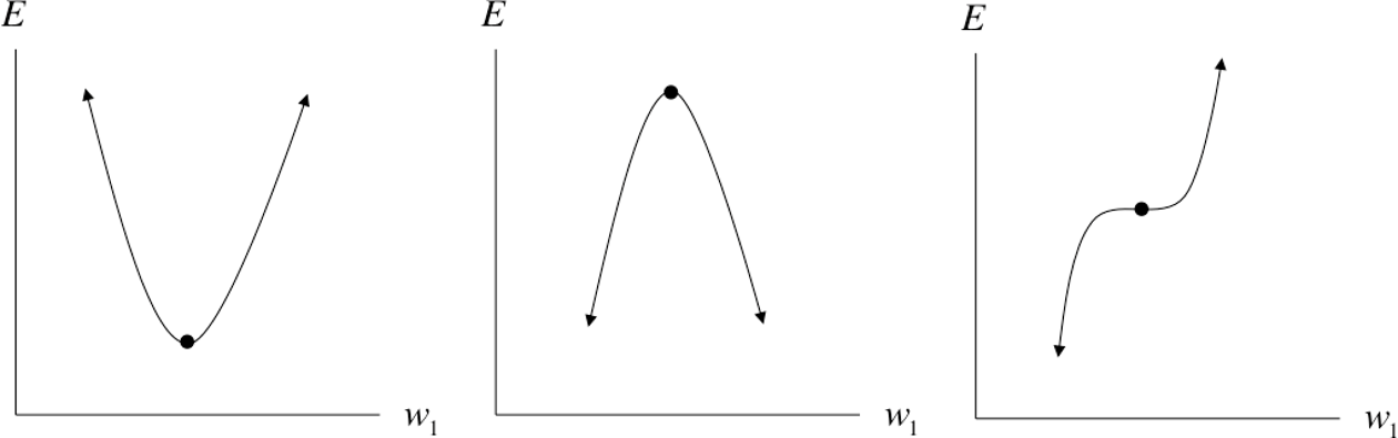
Figure 4-4. Analyzing a critical point along a single dimension
We can also extend this to higher dimensional functions. Consider a cost function operating in a -dimensional space. Let’s take an arbitrary critical point. It turns out that figuring out if this point is a local minimum, local maximum, or a saddle point is a little bit trickier than in the one-dimensional case. Consider the error surface in Figure 4-5. Depending on how you slice the surface (from A to B or from C to D), the critical point looks like either a minimum or a maximum. In reality, it’s neither. It’s a more complex type of saddle point.
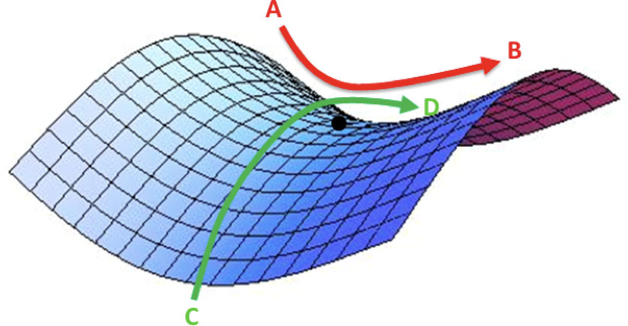
Figure 4-5. A saddle point over a two-dimensional error surface
In general, in a -dimensional parameter space, we can slice through a critical point on different axes. A critical point can only be a local minimum if it appears as a local minimum in every single one of the one-dimensional subspaces. Using the fact that a critical point can come in one of three different flavors in a one-dimensional subspace, we realize that the probability that a random critical point is in a random function is . This means that a random function function with critical points has an expected number of local minima. In other words, as the dimensionality of our parameter space increases, local minima become exponentially more rare. A more rigorous treatment of this topic is outside the scope of this book, but is explored more extensively by Dauphin et al. in 2014.3
So what does this mean for optimizing deep learning models? For stochastic gradient descent, it’s still unclear. It seems like these flat segments of the error surface are pesky but ultimately don’t prevent stochastic gradient descent from converging to a good answer. However, it does pose serious problems for methods that attempt to directly solve for a point where the gradient is zero. This has been a major hindrance to the usefulness of certain second-order optimization methods for deep learning models, which we will discuss later.
When the Gradient Points in the Wrong Direction
Upon analyzing the error surfaces of deep networks, it seems like the most critical challenge to optimizing deep networks is finding the correct trajectory to move in. It’s no surprise, however, that this is a major challenge when we look at what happens to the error surface around a local minimum. As an example, we consider an error surface defined over a two-dimensional parameter space, as shown in Figure 4-6.
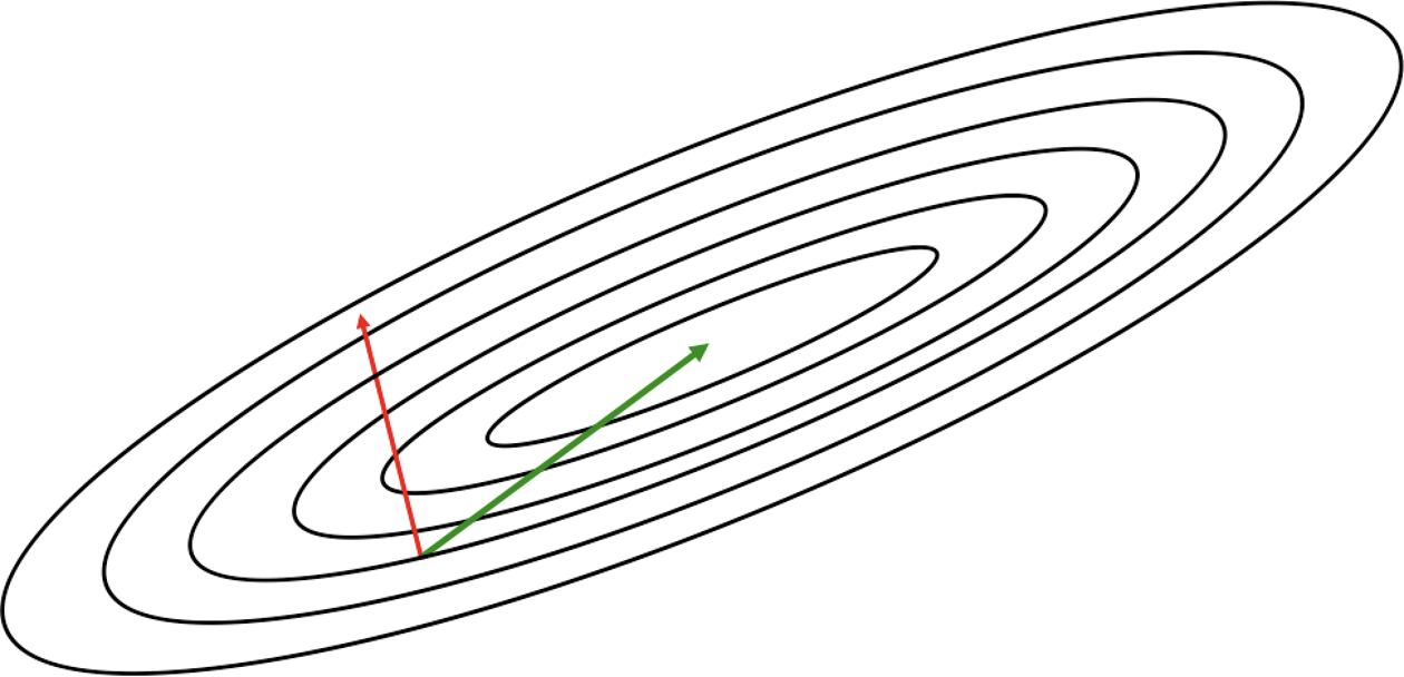
Figure 4-6. Local information encoded by the gradient usually does not corroborate the global structure of the error surface
Revisiting the contour diagrams we explored in Chapter 2, we notice that the gradient isn’t usually a very good indicator of the good trajectory. Specifically, we realize that only when the contours are perfectly circular does the gradient always point in the direction of the local minimum. However, if the contours are extremely elliptical (as is usually the case for the error surfaces of deep networks), the gradient can be as inaccurate as 90 degrees away from the correct direction!
We extend this analysis to an arbitrary number of dimensions using some mathematical formalism. For every weight in the parameter space, the gradient computes the value of , or how the value of the error changes as we change the value of . Taken together over all weights in the parameter space, the gradient gives us the direction of steepest descent. The general problem with taking a significant step in this direction, however, is that the gradient could be changing under our feet as we move! We demonstrate this simple fact in Figure 4-7. Going back to the two-dimensional example, if our contours are perfectly circular and we take a big step in the direction of the steepest descent, the gradient doesn’t change direction as we move. However, this is not the case for highly elliptical contours.
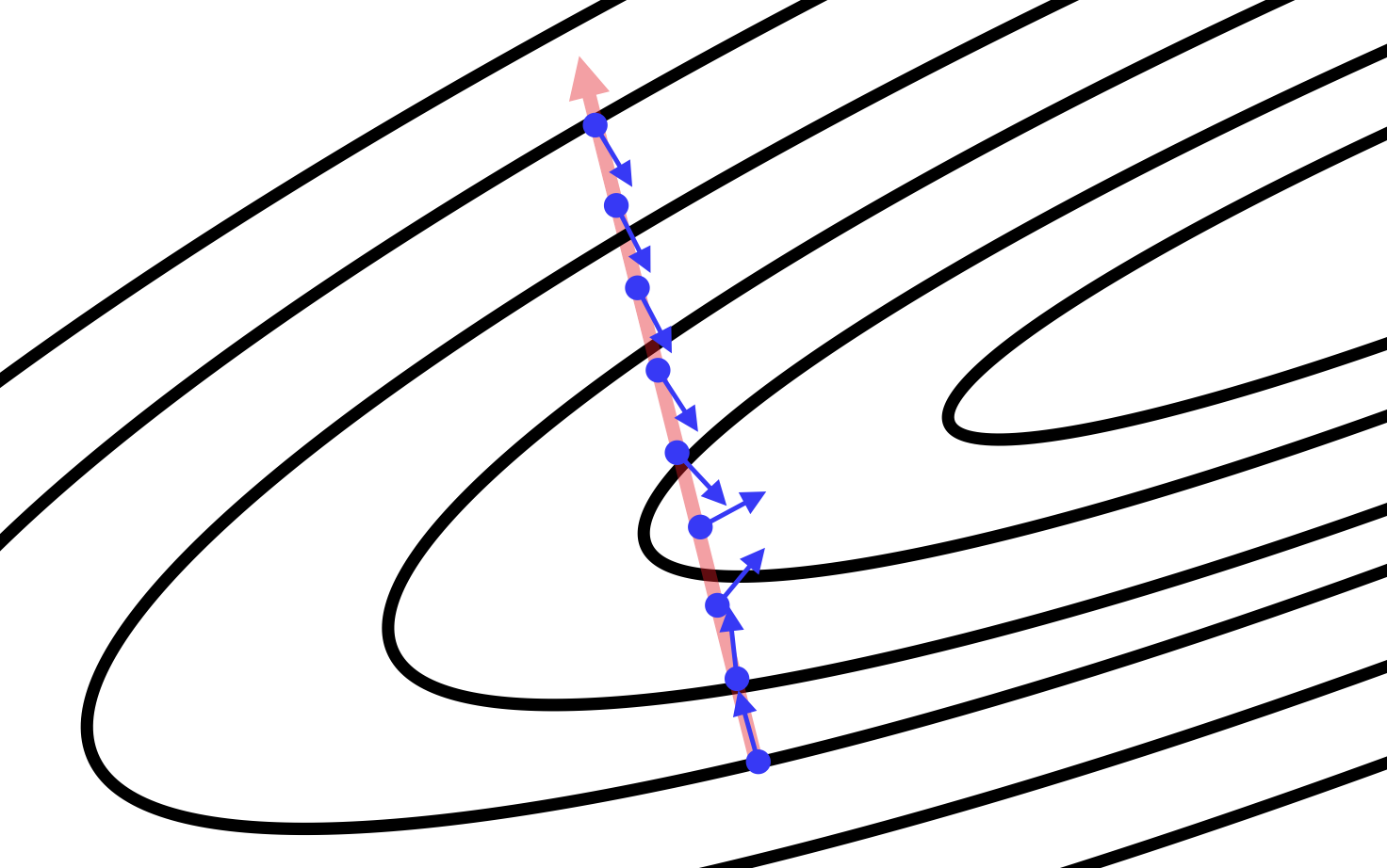
Figure 4-7. We show how the direction of the gradient changes as we move along the direction of steepest descent (as determined from a starting point). The gradient vectors are normalized to identical length to emphasize the change in direction of the gradient vector.
More generally, we can quantify how the gradient changes under our feet as we move in a certain direction by computing second derivatives. Specifically, we want to measure , which tells us how the gradient component for changes as we change the value of . We can compile this information into a special matrix known as the Hessian matrix (H). And when describing an error surface where the gradient changes underneath our feet as we move in the direction of steepest descent, this matrix is said to be ill-conditioned.
For the mathematically inclined reader, we go into slightly more detail about how the Hessian limits optimization purely by gradient descent. Certain properties of the Hessian matrix (specifically that it is real and symmetric) allow us to efficiently determine the second derivative (which approximates the curvature of a surface) as we move in a specific direction. Specifically, if we have a unit vector d, the second derivative in that direction is given by dHd. We can now use a second-order approximation via Taylor series to understand what happens to the error function as we step from the current parameter vector x(i) to a new parameter vector x along gradient vector g evaluated at x(i):
If we go further to state that we will be moving units in the direction of the gradient, we can further simplify our expression:
Hg
This expression consists of three terms: 1) the value of the error function at the original parameter vector, 2) the improvement in error afforded by the magnitude of the gradient, and 3) a correction term that incorporates the curvature of the surface as represented by the Hessian matrix.
In general, we should be able to use this information to design better optimization algorithms. For instance, we can even naively take the second order approximation of the error function to determine the learning rate at each step that maximizes the reduction in the error function. It turns out, however, that computing the Hessian matrix exactly is a difficult task. In the next several sections, we’ll describe optimization breakthroughs that tackle ill-conditioning without directly computing the Hessian matrix.
Momentum-Based Optimization
Fundamentally, the problem of an ill-conditioned Hessian matrix manifests itself in the form of gradients that fluctuate wildly. As a result, one popular mechanism for dealing with ill-conditioning bypasses the computation of the Hessian, and instead, focuses on how to cancel out these fluctuations over the duration of training.
One way to think about how we might tackle this problem is by investigating how a ball rolls down a hilly surface. Driven by gravity, the ball eventually settles into a minimum on the surface, but for some reason, it doesn’t suffer from the wild fluctuations and divergences that happen during gradient descent. Why is this the case? Unlike in stochastic gradient descent (which only uses the gradient), there are two major components that determine how a ball rolls down an error surface. The first, which we already model in SGD as the gradient, is what we commonly refer to as acceleration. But acceleration does not single-handedly determine the ball’s movements. Instead, its motion is more directly determined by its velocity. Acceleration only indirectly changes the ball’s position by modifying its velocity.
Velocity-driven motion is desirable because it counteracts the effects of a wildly fluctuating gradient by smoothing the ball’s trajectory over its history. Velocity serves as a form of memory, and this allows us to more effectively accumulate movement in the direction of the minimum while canceling out oscillating accelerations in orthogonal directions. Our goal, then, is to somehow generate an analog for velocity in our optimization algorithm. We can do this by keeping track of an exponentially weighted decay of past gradients. The premise is simple: every update is computed by combining the update in the last iteration with the current gradient. Concretely, we compute the change in the parameter vector as follows:
In other words, we use the momentum hyperparameter to determine what fraction of the previous velocity to retain in the new update, and add this “memory” of past gradients to our current gradient. This approach is commonly referred to as momentum.4 Because the momentum term increases the step size we take, using momentum may require a reduced learning rate compared to vanilla stochastic gradient descent.
To better visualize how momentum works, we’ll explore a toy example. Specifically, we’ll investigate how momentum affects updates during a random walk. A random walk is a succession of randomly chosen steps. In our example, we’ll imagine a particle on a line that, at every time interval, randomly picks a step size between -10 and 10 and takes a moves in that direction. This is simply expressed as:
step_range = 10
step_range = 10step_choices = range(-1 * step_range,
                                         step_range + 1)
rand_walk = [random.choice(step_choices) for x in xrange(100)]
We’ll then simulate what happens when we use a slight modification of momentum (i.e., the standard exponentially weighted moving average algorithm) to smooth our choice of step at every time interval. Again, we can concisely express this as:
momentum_rand_walk = [random.choice(step_choices)]
for i in xrange(len(rand_walk) - 1):
    prev = momentum_rand_walk[-1]
    rand_choice = random.choice(step_choices)
    new_step = momentum * prev + (1 - momentum) * rand_choice
    momentum_rand_walk.append()
The results, as we vary the momentum from 0 to 1, are quite staggering. Momentum significantly reduces the volatility of updates. The larger the momentum, the less responsive we are to new updates (e.g., a large inaccuracy on the first estimation of trajectory propagates for a significant period of time). We summarize the results of our toy experiment in Figure 4-8.

Figure 4-8. Momentum smooths volatility in the step sizes during a random walk using an exponentially weighted moving average
To investigate how momentum actually affects the training of feedforward neural networks, we can retrain our trusty MNIST feedforward network with a TensorFlow momentum optimizer. In this case we can get away with using the same learning rate (0.01) with a typical momentum of 0.9:
learning_rate = 0.01
momentum = 0.9
optimizer = tf.train.MomentumOptimizer(learning_rate, momentum)
train_op = optimizer.minimize(cost, global_step=global_step)
The resulting speedup is staggering. We display how the cost function changes over time by comparing the TensorBoard visualizations in Figure 4-9. The figure demonstrates that to achieve a cost of 0.1 without momentum (right) requires nearly 18,000 steps (minibatches), whereas with momentum (left), we require just over 2,000.

Figure 4-9. Comparing training a feed-forward network with (right) and without (left) momentum demonstrates a massive decrease in training time
Recently, more work has been done exploring how the classical momentum technique can be improved. Sutskever et al. in 2013 proposed an alternative called Nesterov momentum, which computes the gradient on the error surface at during the velocity update instead of at .5 This subtle difference seems to allow Nesterov momentum to change its velocity in a more responsive way. It’s been shown that this method has clear benefits in batch gradient descent (convergence guarantees and the ability to use a higher momentum for a given learning rate as compared to classical momentum), but it’s not entirely clear whether this is true for the more stochastic mini-batch gradient descent used in most deep learning optimization approaches. Support for Nerestov momentum is not yet available out of the box in TensorFlow as of the writing of this text.
A Brief View of Second-Order Methods
As we discussed in previous sections, computing the Hessian is a computationally difficult task, and momentum afforded us significant speedup without having to worry about it altogether. Several second-order methods, however, have been researched over the past several years that attempt to approximate the Hessian directly. For completeness, we give a broad overview of these methods, but a detailed treatment is beyond the scope of this text.
The first is conjugate gradient descent, which arises out of attempting to improve on a naive method of steepest descent. In steepest descent, we compute the direction of the gradient and then line search to find the minimum along that direction. We jump to the minimum and then recompute the gradient to determine the direction of the next line search. It turns out that this method ends up zigzagging a significant amount, as shown in Figure 4-9, because each time we move in the direction of steepest descent, we undo a little bit of progress in another direction. A remedy to this problem is moving in a conjugate direction relative to the previous choice instead of the direction of steepest descent. The conjugate direction is chosen by using an indirect approximation of the Hessian to linearly combine the gradient and our previous direction. With a slight modification, this method generalizes to the nonconvex error surfaces we find in deep networks.6
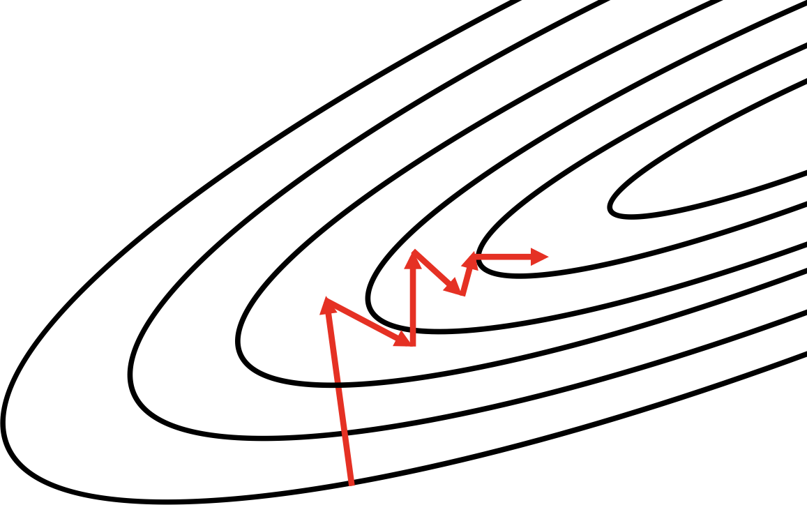
Figure 4-10. The method of steepest descent often zigzags; conjugate descent attempts to remedy this issue
An alternative optimization algorithm known as the Broyden–Fletcher–Goldfarb–Shanno (BFGS) algorithm attempts to compute the inverse of the Hessian matrix iteratively and use the inverse Hessian to more effectively optimize the parameter vector.7 In its original form, BFGS has a significant memory footprint, but recent work has produced a more memory-efficient version known as L-BFGS.8
In general, while these methods hold some promise, second-order methods are still an area of active research and are unpopular among practitioners. TensorFlow does not currently support either conjugate gradient descent or L-BFGS at the time of writing this text, although these features seem to be in the development pipeline.
Learning Rate Adaptation
As we have discussed previously, another major challenge for training deep networks is appropriately selecting the learning rate. Choosing the correct learning rate has long been one of the most troublesome aspects of training deep networks because it has a major impact on a network’s performance. A learning rate that is too small doesn’t learn quickly enough, but a learning rate that is too large may have difficulty converging as we approach a local minimum or region that is ill-conditioned.
One of the major breakthroughs in modern deep network optimization was the advent of learning rate adaption. The basic concept behind learning rate adaptation is that the optimal learning rate is appropriately modified over the span of learning to achieve good convergence properties. Over the next several sections, we’ll discuss AdaGrad, RMSProp, and Adam, three of the most popular adaptive learning rate algorithms.
AdaGrad—Accumulating Historical Gradients
The first algorithm we’ll discuss is AdaGrad, which attempts to adapt the global learning rate over time using an accumulation of the historical gradients, first proposed by Duchi et al. in 2011.9 Specifically, we keep track of a learning rate for each parameter. This learning rate is inversely scaled with respect to the square root of the sum of the squares (root mean square) of all the parameter’s historical gradients.
We can express this mathematically. We initialize a gradient accumulation vector . At every step, we accumulate the square of all the gradient parameters as follows (where the operation is element-wise tensor multiplication):
Then we compute the update as usual, except our global learning rate is divided by the square root of the gradient accumulation vector:
Note that we add a tiny number (~) to the denominator in order to prevent division by zero. Also, the division and addition operations are broadcast to the size of the gradient accumulation vector and applied element-wise. In TensorFlow, a built-in optimizer allows for easily utilizing AdaGrad as a learning algorithm:
tf.train.AdagradOptimizer(learning_rate,
                          initial_accumulator_value=0.1,
                          use_locking=False,
                          name='Adagrad')
The only hitch is that in TensorFlow, the and initial gradient accumulation vector are rolled together into the initial_accumulator_value argument.
On a functional level, this update mechanism means that the parameters with the largest gradients experience a rapid decrease in their learning rates, while parameters with smaller gradients only observe a small decrease in their learning rates. The ultimate effect is that AdaGrad forces more progress in the more gently sloped directions on the error surface, which can help overcome ill-conditioned surfaces. This results in some good theoretical properties, but in practice, training deep learning models with AdaGrad can be somewhat problematic. Empirically, AdaGrad has a tendency to cause a premature drop in learning rate, and as a result doesn’t work particularly well for some deep models. In the next section, we’ll describe RMSProp, which attempts to remedy this shortcoming.
RMSProp—Exponentially Weighted Moving Average of Gradients
While AdaGrad works well for simple convex functions, it isn’t designed to navigate the complex error surfaces of deep networks. Flat regions may force AdaGrad to decrease the learning rate before it reaches a minimum. The conclusion is that simply using a naive accumulation of gradients isn’t sufficient.
Our solution is to bring back a concept we introduced earlier while discussing momentum to dampen fluctuations in the gradient. Compared to naive accumulation, exponentially weighted moving averages also enable us to “toss out” measurements that we made a long time ago. More specifically, our update to the gradient accumulation vector is now as follows:
The decay factor determines how long we keep old gradients. The smaller the decay factor, the shorter the effective window. Plugging this modification into AdaGrad gives rise to the RMSProp learning algorithm, first proposed by Geoffrey Hinton.10
In TensorFlow, we can instantiate the RMSProp optimizer with the following code. We note that in this case, unlike in Adagrad, we pass in separately as the epsilon argument to the constructor:
tf.train.RMSPropOptimizer(learning_rate, decay=0.9,
                          momentum=0.0, epsilon=1e-10,
                          use_locking=False, name='RMSProp')
As the template suggests, we can utilize RMSProp with momentum (specifically Nerestov momentum). Overall, RMSProp has been shown to be a highly effective optimizer for deep neural networks, and is a default choice for many seasoned practitioners.
Adam—Combining Momentum and RMSProp
Before concluding our discussion of modern optimizers, we discuss one final algorithm—Adam.11 Spiritually, we can think about Adam as a variant combination of RMSProp and momentum.
The basic idea is as follows. We want to keep track of an exponentially weighted moving average of the gradient (essentially the concept of velocity in classical momentum), which we can express as follows:
mi = β1mi-1 + (1-β1)gi
This is our approximation of what we call the first moment of the gradient, or 𝔼[gi]. And similarly to RMSProp, we can maintain an exponentially weighted moving average of the historical gradients. This is our estimation of what we call the second moment of the gradient, or 𝔼[gi ⊙ gi]:
However, it turns out these estimations are biased relative to the real moments because we start off by initializing both vectors to the zero vector. In order to remedy this bias, we derive a correction factor for both estimations. Here, we describe the derivation for the estimation of the second moment. The derivation for the first moment, which is analogous to the derivation here, is left as an exercise for the mathematically inclined reader.
We begin by expressing the estimation of the second moment in terms of all past gradients. This is done by simply expanding the recurrence relationship:
We can then take the expected value of both sides to determine how our estimation 𝔼[vi] compares to the real value of 𝔼[gi ⊙ gi]:
𝔼[vi] = 𝔼
We can also assume that 𝔼[gk ⊙ gk] ≈ 𝔼[gi ≈ gi], because even if the second moment of the gradient has changed since a historical value, should be chosen so that the old second moments of the gradients are essentially decayed out of relevancy. As a result, we can make the following simplification:
𝔼[vi] ≈ 𝔼[gi ⊙ gi]
𝔼[vi] ≈ 𝔼[gi ⊙ gi](1-β2i)
Note that we make the final simplification using the elementary algebraic identity . The results of this derivation and the analogous derivation for the first moment are the following correction schemes to account for the initialization bias:
m̃i =
We can then use these corrected moments to update the parameter vector, resulting in the final Adam update:
m̃i
Recently, Adam has gained popularity because of its corrective measures against the zero initialization bias (a weakness of RMSProp) and its ability to combine the core concepts behind RMSProp with momentum more effectively. TensorFlow exposes the Adam optimizer through the following constructor:
tf.train.AdamOptimizer(learning_rate=0.001, beta1=0.9,
                       beta2=0.999, epsilon=1e-08,
                       use_locking=False, name='Adam')
The default hyperparameter settings for Adam for TensorFlow generally perform quite well, but Adam is also generally robust to choices in hyperparameters. The only exception is that the learning rate may need to be modified in certain cases from the default value of 0.001.
The Philosophy Behind Optimizer Selection
In this chapter, we’ve discussed several strategies that are used to make navigating the complex error surfaces of deep networks more tractable. These strategies have culminated in several optimization algorithms, each with its own benefits and shortcomings.
While it would be awfully nice to know when to use which algorithm, there is very little consensus among expert practitioners. Currently, the most popular algorithms are mini-batch gradient descent, mini-batch gradient with momentum, RMSProp, RMSProp with momentum, Adam, and AdaDelta (which we haven’t discussed here, and is not currently supported by TensorFlow as of the writing of this text). We include a TensorFlow script in the Github repository for this text for the curious reader to experiment with these optimization algorithms on the feed-forward network model we built:
$ python optimzer_mlp.py <sgd, momentum, adagrad, rmsprop,
   adam>
One important point, however, is that for most deep learning practitioners, the best way to push the cutting edge of deep learning is not by building more advanced optimizers. Instead, the vast majority of breakthroughs in deep learning over the past several decades have been obtained by discovering architectures that are easier to train instead of trying to wrangle with nasty error surfaces. We’ll begin focusing on how to leverage architecture to more effectively train neural networks in the rest of this book.
Summary
In this chapter, we discussed several challenges that arise when trying to train deep networks with complex error surfaces. We discussed how while the challenges of spurious local minima may likely be exaggerated, saddle points and ill-conditioning do pose a serious threat to the success of vanilla mini-batch gradient descent. We described how momentum can be used to overcome ill-conditioning, and briefly discussed recent research in second-order methods to approximate the Hessian matrix. We also described the evolution of adaptive learning rate optimizers, which tune the learning rate during the training process for better convergence.
In the next chapter, we’ll begin tackling the larger issue of network architecture and design. We’ll begin by exploring computer vision and how we might design deep networks that learn effectively from complex images.
1 Bengio, Yoshua, et al. “Greedy Layer-Wise Training of Deep Networks.” Advances in Neural Information Processing Systems 19 (2007): 153.
2 Goodfellow, Ian J., Oriol Vinyals, and Andrew M. Saxe. “Qualitatively characterizing neural network optimization problems.” arXiv preprint arXiv:1412.6544 (2014).
3 Dauphin, Yann N., et al. “Identifying and attacking the saddle point problem in high-dimensional non-convex optimization.” Advances in Neural Information Processing Systems. 2014.
4 Polyak, Boris T. “Some methods of speeding up the convergence of iteration methods.” USSR Computational Mathematics and Mathematical Physics 4.5 (1964): 1-17.
5 Sutskever, Ilya, et al. “On the importance of initialization and momentum in deep learning.” ICML (3) 28 (2013): 1139-1147.
6 Møller, Martin Fodslette. “A Scaled Conjugate Gradient Algorithm for Fast Supervised Learning.” Neural Networks 6.4 (1993): 525-533.
7 Broyden, C. G. “A new method of solving nonlinear simultaneous equations.” The Computer Journal 12.1 (1969): 94-99.
8 Bonnans, Joseph-Frédéric, et al. Numerical Optimization: Theoretical and Practical Aspects. Springer Science & Business Media, 2006.
9 Duchi, John, Elad Hazan, and Yoram Singer. “Adaptive Subgradient Methods for Online Learning and Stochastic Optimization.” Journal of Machine Learning Research 12.Jul (2011): 2121-2159.
10 Tieleman, Tijmen, and Geoffrey Hinton. “Lecture 6.5-rmsprop: Divide the gradient by a running average of its recent magnitude.” COURSERA: Neural Networks for Machine Learning 4.2 (2012).
11 Kingma, Diederik, and Jimmy Ba. “Adam: A Method for Stochastic Optimization.” arXiv preprint arXiv:1412.6980 (2014).
Get Fundamentals of Deep Learning now with the O’Reilly learning platform.
O’Reilly members experience books, live events, courses curated by job role, and more from O’Reilly and nearly 200 top publishers.

