Chapter 1. The Neural Network
Building Intelligent Machines
The brain is the most incredible organ in the human body. It dictates the way we perceive every sight, sound, smell, taste, and touch. It enables us to store memories, experience emotions, and even dream. Without it, we would be primitive organisms, incapable of anything other than the simplest of reflexes. The brain is, inherently, what makes us intelligent.
The infant brain only weighs a single pound, but somehow it solves problems that even our biggest, most powerful supercomputers find impossible. Within a matter of months after birth, infants can recognize the faces of their parents, discern discrete objects from their backgrounds, and even tell apart voices. Within a year, they’ve already developed an intuition for natural physics, can track objects even when they become partially or completely blocked, and can associate sounds with specific meanings. And by early childhood, they have a sophisticated understanding of grammar and thousands of words in their vocabularies.1
For decades, we’ve dreamed of building intelligent machines with brains like ours—robotic assistants to clean our homes, cars that drive themselves, microscopes that automatically detect diseases. But building these artificially intelligent machines requires us to solve some of the most complex computational problems we have ever grappled with; problems that our brains can already solve in a manner of microseconds. To tackle these problems, we’ll have to develop a radically different way of programming a computer using techniques largely developed over the past decade. This is an extremely active field of artificial computer intelligence often referred to as deep learning.
The Limits of Traditional Computer Programs
Why exactly are certain problems so difficult for computers to solve? Well, it turns out that traditional computer programs are designed to be very good at two things: 1) performing arithmetic really fast and 2) explicitly following a list of instructions. So if you want to do some heavy financial number crunching, you’re in luck. Traditional computer programs can do the trick. But let’s say we want to do something slightly more interesting, like write a program to automatically read someone’s handwriting. Figure 1-1 will serve as a starting point.
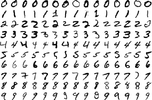
Figure 1-1. Image from MNIST handwritten digit dataset2
Although every digit in Figure 1-1 is written in a slightly different way, we can easily recognize every digit in the first row as a zero, every digit in the second row as a one, etc. Let’s try to write a computer program to crack this task. What rules could we use to tell one digit from another?
Well, we can start simple! For example, we might state that we have a zero if our image only has a single, closed loop. All the examples in Figure 1-1 seem to fit this bill, but this isn’t really a sufficient condition. What if someone doesn’t perfectly close the loop on their zero? And, as in Figure 1-2, how do you distinguish a messy zero from a six?

Figure 1-2. A zero that’s algorithmically difficult to distinguish from a six
You could potentially establish some sort of cutoff for the distance between the starting point of the loop and the ending point, but it’s not exactly clear where we should be drawing the line. But this dilemma is only the beginning of our worries. How do we distinguish between threes and fives? Or between fours and nines? We can add more and more rules, or features, through careful observation and months of trial and error, but it’s quite clear that this isn’t going to be an easy process.
Many other classes of problems fall into this same category: object recognition, speech comprehension, automated translation, etc. We don’t know what program to write because we don’t know how it’s done by our brains. And even if we did know how to do it, the program might be horrendously complicated.
The Mechanics of Machine Learning
To tackle these classes of problems, we’ll have to use a very different kind of approach. A lot of the things we learn in school growing up have a lot in common with traditional computer programs. We learn how to multiply numbers, solve equations, and take derivatives by internalizing a set of instructions. But the things we learn at an extremely early age, the things we find most natural, are learned by example, not by formula.
For instance, when we were two years old, our parents didn’t teach us how to recognize a dog by measuring the shape of its nose or the contours of its body. We learned to recognize a dog by being shown multiple examples and being corrected when we made the wrong guess. In other words, when we were born, our brains provided us with a model that described how we would be able to see the world. As we grew up, that model would take in our sensory inputs and make a guess about what we were experiencing. If that guess was confirmed by our parents, our model would be reinforced. If our parents said we were wrong, we’d modify our model to incorporate this new information. Over our lifetime, our model becomes more and more accurate as we assimilate more and more examples. Obviously all of this happens subconsciously, without us even realizing it, but we can use this to our advantage nonetheless.
Deep learning is a subset of a more general field of artificial intelligence called machine learning, which is predicated on this idea of learning from example. In machine learning, instead of teaching a computer a massive list of rules to solve the problem, we give it a model with which it can evaluate examples, and a small set of instructions to modify the model when it makes a mistake. We expect that, over time, a well-suited model would be able to solve the problem extremely accurately.
Let’s be a little bit more rigorous about what this means so we can formulate this idea mathematically. Let’s define our model to be a function . The input x is an example expressed in vector form. For example, if x were a grayscale image, the vector’s components would be pixel intensities at each position, as shown in Figure 1-3.
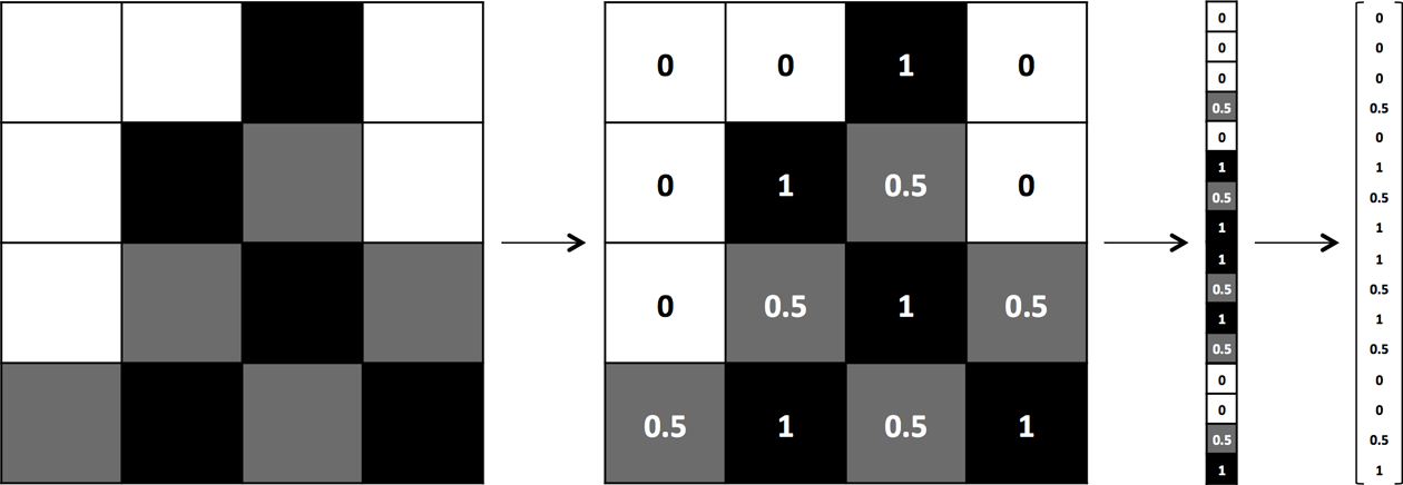
Figure 1-3. The process of vectorizing an image for a machine learning algorithm
The input is a vector of the parameters that our model uses. Our machine learning program tries to perfect the values of these parameters as it is exposed to more and more examples. We’ll see this in action and in more detail in Chapter 2.
To develop a more intuitive understanding for machine learning models, let’s walk through a quick example. Let’s say we wanted to determine how to predict exam performance based on the number of hours of sleep we get and the number of hours we study the previous day. We collect a lot of data, and for each data point , we record the number of hours of sleep we got (), the number of hours we spent studying (), and whether we performed above or below the class average. Our goal, then, might be to learn a model with parameter vector such that:
In other words, we guess that the blueprint for our model is as described above (geometrically, this particular blueprint describes a linear classifier that divides the coordinate plane into two halves). Then, we want to learn a parameter vector such that our model makes the right predictions (−1 if we perform below average, and 1 otherwise) given an input example x. This model is called a linear perceptron, and it’s a model that’s been used since the 1950s.3 Let’s assume our data is as shown in Figure 1-4.
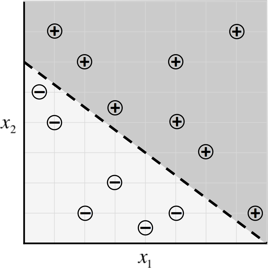
Figure 1-4. Sample data for our exam predictor algorithm and a potential classifier
Then it turns out, by selecting , our machine learning model makes the correct prediction on every data point:
An optimal parameter vector positions the classifier so that we make as many correct predictions as possible. In most cases, there are many (or even infinitely many) possible choices for that are optimal. Fortunately for us, most of the time these alternatives are so close to one another that the difference is negligible. If this is not the case, we may want to collect more data to narrow our choice of .
While the setup seems reasonable, there are still some pretty significant questions that remain. First off, how do we even come up with an optimal value for the parameter vector in the first place? Solving this problem requires a technique commonly known as optimization. An optimizer aims to maximize the performance of a machine learning model by iteratively tweaking its parameters until the error is minimized. We’ll begin to tackle this question of learning parameter vectors in more detail in Chapter 2, when we describe the process of gradient descent.4 In later chapters, we’ll try to find ways to make this process even more efficient.
Second, it’s quite clear that this particular model (the linear perceptron model) is quite limited in the relationships it can learn. For example, the distributions of data shown in Figure 1-5 cannot be described well by a linear perceptron.
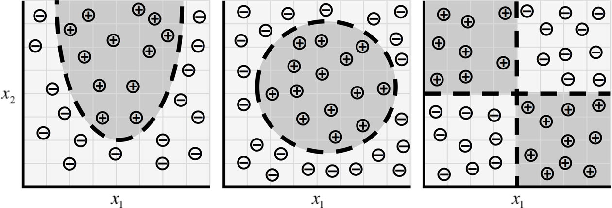
Figure 1-5. As our data takes on more complex forms, we need more complex models to describe them
But these situations are only the tip of the iceberg. As we move on to much more complex problems, such as object recognition and text analysis, our data becomes extremely high dimensional, and the relationships we want to capture become highly nonlinear. To accommodate this complexity, recent research in machine learning has attempted to build models that resemble the structures utilized by our brains. It’s essentially this body of research, commonly referred to as deep learning, that has had spectacular success in tackling problems in computer vision and natural language processing. These algorithms not only far surpass other kinds of machine learning algorithms, but also rival (or even exceed!) the accuracies achieved by humans.
The Neuron
The foundational unit of the human brain is the neuron. A tiny piece of the brain, about the size of grain of rice, contains over 10,000 neurons, each of which forms an average of 6,000 connections with other neurons.5 It’s this massive biological network that enables us to experience the world around us. Our goal in this section will be to use this natural structure to build machine learning models that solve problems in an analogous way.
At its core, the neuron is optimized to receive information from other neurons, process this information in a unique way, and send its result to other cells. This process is summarized in Figure 1-6. The neuron receives its inputs along antennae-like structures called dendrites. Each of these incoming connections is dynamically strengthened or weakened based on how often it is used (this is how we learn new concepts!), and it’s the strength of each connection that determines the contribution of the input to the neuron’s output. After being weighted by the strength of their respective connections, the inputs are summed together in the cell body. This sum is then transformed into a new signal that’s propagated along the cell’s axon and sent off to other neurons.
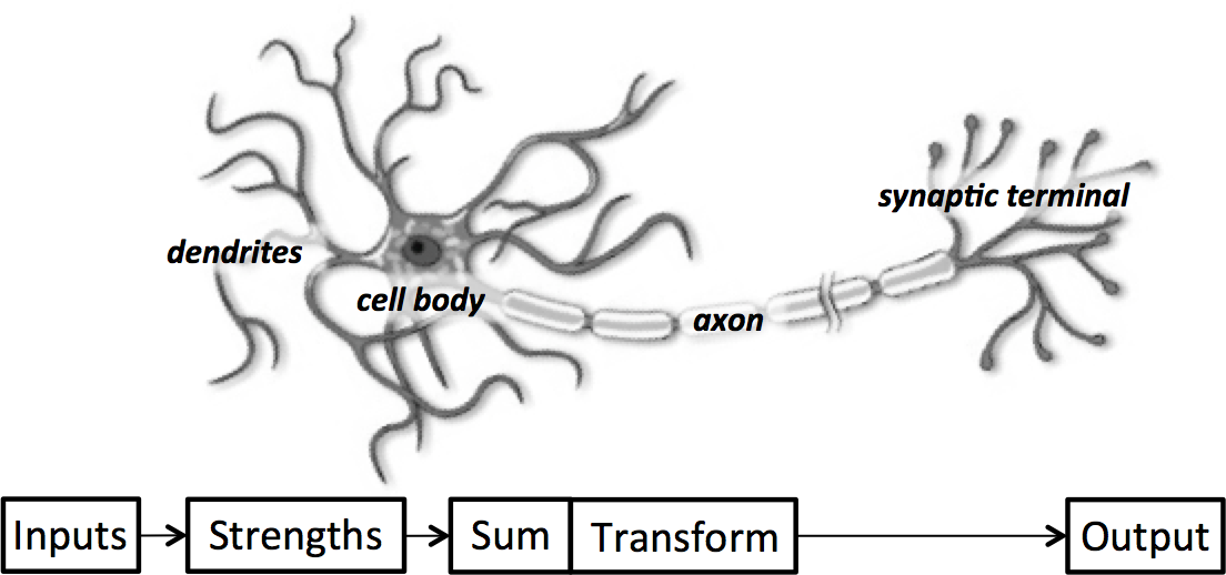
Figure 1-6. A functional description of a biological neuron’s structure
We can translate this functional understanding of the neurons in our brain into an artificial model that we can represent on our computer. Such a model is described in Figure 1-7, leveraging the approach first pioneered in 1943 by Warren S. McCulloch and Walter H. Pitts.6 Just as in biological neurons, our artificial neuron takes in some number of inputs, , each of which is multiplied by a specific weight, . These weighted inputs are, as before, summed together to produce the logit of the neuron, . In many cases, the logit also includes a bias, which is a constant (not shown in the figure). The logit is then passed through a function to produce the output . This output can be transmitted to other neurons.
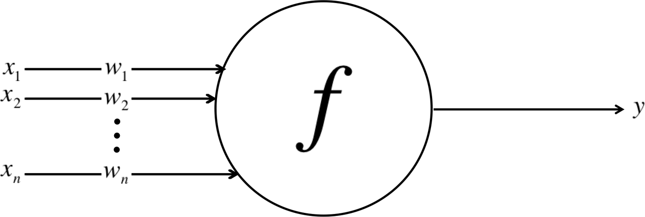
Figure 1-7. Schematic for a neuron in an artificial neural net
We’ll conclude our mathematical discussion of the artificial neuron by re-expressing its functionality in vector form. Let’s reformulate the inputs as a vector x = [x1 x2 ... xn] and the weights of the neuron as w = [w1 w2 ... wn]. Then we can re-express the output of the neuron as , where is the bias term. In other words, we can compute the output by performing the dot product of the input and weight vectors, adding in the bias term to produce the logit, and then applying the transformation function. While this seems like a trivial reformulation, thinking about neurons as a series of vector manipulations will be crucial to how we implement them in software later in this book.
Expressing Linear Perceptrons as Neurons
In “The Mechanics of Machine Learning”, we talked about using machine learning models to capture the relationship between success on exams and time spent studying and sleeping. To tackle this problem, we constructed a linear perceptron classifier that divided the Cartesian coordinate plane into two halves:
As shown in Figure 1-4, this is an optimal choice for because it correctly classifies every sample in our dataset. Here, we show that our model h is easily using a neuron. Consider the neuron depicted in Figure 1-8. The neuron has two inputs, a bias, and uses the function:
It’s very easy to show that our linear perceptron and the neuronal model are perfectly equivalent. And in general, it’s quite simple to show that singular neurons are strictly more expressive than linear perceptrons. In other words, every linear perceptron can be expressed as a single neuron, but single neurons can also express models that cannot be expressed by any linear perceptron.
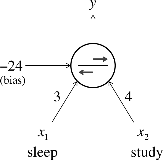
Figure 1-8. Expressing our exam performance perceptron as a neuron
Feed-Forward Neural Networks
Although single neurons are more powerful than linear perceptrons, they’re not nearly expressive enough to solve complicated learning problems. There’s a reason our brain is made of more than one neuron. For example, it is impossible for a single neuron to differentiate handwritten digits. So to tackle much more complicated tasks, we’ll have to take our machine learning model even further.
The neurons in the human brain are organized in layers. In fact, the human cerebral cortex (the structure responsible for most of human intelligence) is made up of six layers.7 Information flows from one layer to another until sensory input is converted into conceptual understanding. For example, the bottommost layer of the visual cortex receives raw visual data from the eyes. This information is processed by each layer and passed on to the next until, in the sixth layer, we conclude whether we are looking at a cat, or a soda can, or an airplane. Figure 1-9 shows a more simplified version of these layers.
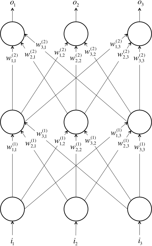
Figure 1-9. A simple example of a feed-forward neural network with three layers (input, one hidden, and output) and three neurons per layer
Borrowing from these concepts, we can construct an artificial neural network. A neural network comes about when we start hooking up neurons to each other, the input data, and to the output nodes, which correspond to the network’s answer to a learning problem. Figure 1-9 demonstrates a simple example of an artificial neural network, similar to the architecture described in McCulloch and Pitt’s work in 1943. The bottom layer of the network pulls in the input data. The top layer of neurons (output nodes) computes our final answer. The middle layer(s) of neurons are called the hidden layers, and we let be the weight of the connection between the neuron in the layer with the neuron in the layer. These weights constitute our parameter vector, , and just as before, our ability to solve problems with neural networks depends on finding the optimal values to plug into .
We note that in this example, connections only traverse from a lower layer to a higher layer. There are no connections between neurons in the same layer, and there are no connections that transmit data from a higher layer to a lower layer. These neural networks are called feed-forward networks, and we start by discussing these networks because they are the simplest to analyze. We present this analysis (specifically, the process of selecting the optimal values for the weights) in Chapter 2. More complicated connectivities will be addressed in later chapters.
In the final sections, we’ll discuss the major types of layers that are utilized in feed-forward neural networks. But before we proceed, here’s a couple of important notes to keep in mind:
- As we mentioned, the layers of neurons that lie sandwiched between the first layer of neurons (input layer) and the last layer of neurons (output layer) are called the hidden layers. This is where most of the magic is happening when the neural net tries to solve problems. Whereas (as in the handwritten digit example) we would previously have to spend a lot of time identifying useful features, the hidden layers automate this process for us. Oftentimes, taking a look at the activities of hidden layers can tell you a lot about the features the network has automatically learned to extract from the data.
- Although in this example every layer has the same number of neurons, this is neither necessary nor recommended. More often than not, hidden layers have fewer neurons than the input layer to force the network to learn compressed representations of the original input. For example, while our eyes obtain raw pixel values from our surroundings, our brain thinks in terms of edges and contours. This is because the hidden layers of biological neurons in our brain force us to come up with better representations for everything we perceive.
- It is not required that every neuron has its output connected to the inputs of all neurons in the next layer. In fact, selecting which neurons to connect to which other neurons in the next layer is an art that comes from experience. We’ll discuss this issue in more depth as we work through various examples of neural networks.
- The inputs and outputs are vectorized representations. For example, you might imagine a neural network where the inputs are the individual pixel RGB values in an image represented as a vector (refer to Figure 1-3). The last layer might have two neurons that correspond to the answer to our problem: if the image contains a dog, if the image contains a cat, if it contains both, and if it contains neither.
We’ll also observe that, similarly to our reformulation for the neuron, we can also mathematically express a neural network as a series of vector and matrix operations. Let’s consider the input to the layer of the network to be a vector x = [x1 x2 ... xn]. We’d like to find the vector y = [y1 y2 ... ym] produced by propagating the input through the neurons. We can express this as a simple matrix multiply if we construct a weight matrix of size and a bias vector of size . In this matrix, each column corresponds to a neuron, where the element of the column corresponds to the weight of the connection pulling in the element of the input. In other words, y = ƒ(WTx + b), where the transformation function is applied to the vector element-wise. This reformulation will become all the more critical as we begin to implement these networks in software.
Linear Neurons and Their Limitations
Most neuron types are defined by the function they apply to their logit . Let’s first consider layers of neurons that use a linear function in the form of . For example, a neuron that attempts to estimate a cost of a meal in a fast-food restaurant would use a linear neuron where and . In other words, using and weights equal to the price of each item, the linear neuron in Figure 1-10 would take in some ordered triple of servings of burgers, fries, and sodas and output the price of the combination.
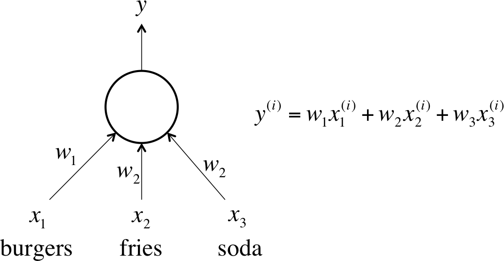
Figure 1-10. An example of a linear neuron
Linear neurons are easy to compute with, but they run into serious limitations. In fact, it can be shown that any feed-forward neural network consisting of only linear neurons can be expressed as a network with no hidden layers. This is problematic because, as we discussed before, hidden layers are what enable us to learn important features from the input data. In other words, in order to learn complex relationships, we need to use neurons that employ some sort of nonlinearity.
Sigmoid, Tanh, and ReLU Neurons
There are three major types of neurons that are used in practice that introduce nonlinearities in their computations. The first of these is the sigmoid neuron, which uses the function:
Intuitively, this means that when the logit is very small, the output of a logistic neuron is very close to 0. When the logit is very large, the output of the logistic neuron is close to 1. In-between these two extremes, the neuron assumes an S-shape, as shown in Figure 1-11.
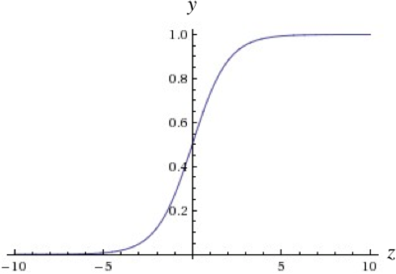
Figure 1-11. The output of a sigmoid neuron as z varies
Tanh neurons use a similar kind of S-shaped nonlinearity, but instead of ranging from 0 to 1, the output of tanh neurons range from −1 to 1. As one would expect, they use . The resulting relationship between the output and the logit is described by Figure 1-12. When S-shaped nonlinearities are used, the tanh neuron is often preferred over the sigmoid neuron because it is zero-centered.
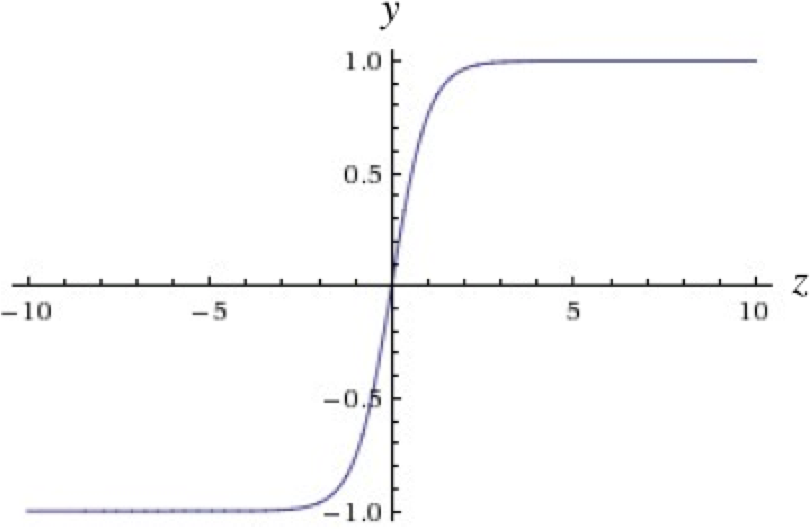
Figure 1-12. The output of a tanh neuron as z varies
A different kind of nonlinearity is used by the restricted linear unit (ReLU) neuron. It uses the function , resulting in a characteristic hockey-stick-shaped response, as shown in Figure 1-13.
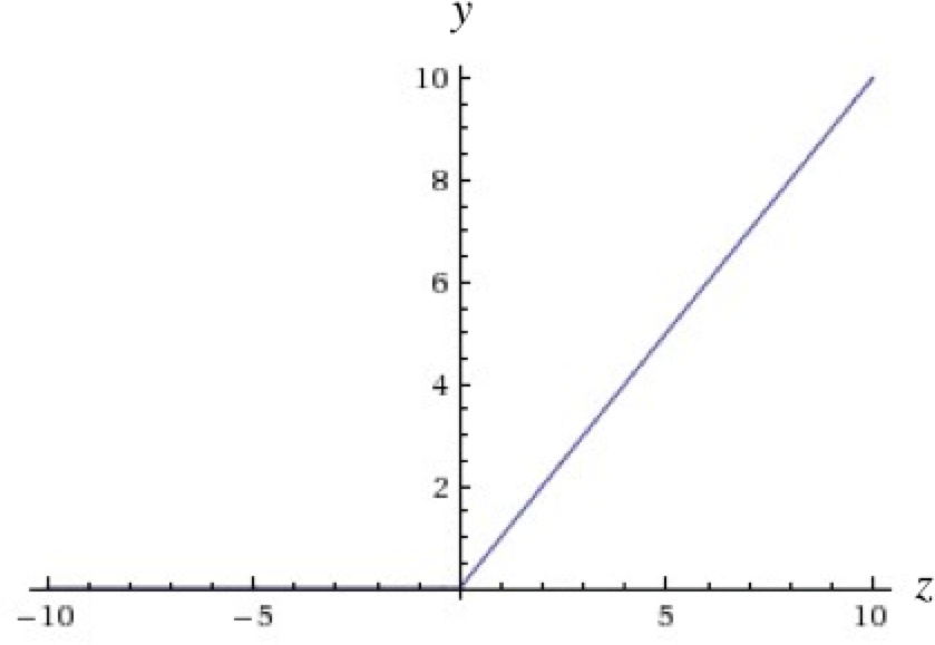
Figure 1-13. The output of a ReLU neuron as z varies
The ReLU has recently become the neuron of choice for many tasks (especially in computer vision) for a number of reasons, despite some drawbacks.8 We’ll discuss these reasons in Chapter 5, as well as strategies to combat the potential pitfalls.
Softmax Output Layers
Oftentimes, we want our output vector to be a probability distribution over a set of mutually exclusive labels. For example, let’s say we want to build a neural network to recognize handwritten digits from the MNIST dataset. Each label (0 through 9) is mutually exclusive, but it’s unlikely that we will be able to recognize digits with 100% confidence. Using a probability distribution gives us a better idea of how confident we are in our predictions. As a result, the desired output vector is of the form below, where :
This is achieved by using a special output layer called a softmax layer. Unlike in other kinds of layers, the output of a neuron in a softmax layer depends on the outputs of all the other neurons in its layer. This is because we require the sum of all the outputs to be equal to 1. Letting be the logit of the softmax neuron, we can achieve this normalization by setting its output to:
A strong prediction would have a single entry in the vector close to 1, while the remaining entries were close to 0. A weak prediction would have multiple possible labels that are more or less equally likely.
Looking Forward
In this chapter, we’ve built a basic intuition for machine learning and neural networks. We’ve talked about the basic structure of a neuron, how feed-forward neural networks work, and the importance of nonlinearity in tackling complex learning problems. In the next chapter, we will begin to build the mathematical background necessary to train a neural network to solve problems. Specifically, we will talk about finding optimal parameter vectors, best practices while training neural networks, and major challenges. In future chapters, we will take these foundational ideas to build more specialized neural architectures.
1 Kuhn, Deanna, et al. Handbook of Child Psychology. Vol. 2, Cognition, Perception, and Language. Wiley, 1998.
2 Y. LeCun, L. Bottou, Y. Bengio, and P. Haffner. “Gradient-Based Learning Applied to Document Recognition” Proceedings of the IEEE, 86(11):2278-2324, November 1998.
3 Rosenblatt, Frank. “The perceptron: A probabilistic model for information storage and organization in the brain.” Psychological Review 65.6 (1958): 386.
4 Bubeck, Sébastien. “Convex optimization: Algorithms and complexity.” Foundations and Trends® in Machine Learning. 8.3-4 (2015): 231-357.
5 Restak, Richard M. and David Grubin. The Secret Life of the Brain. Joseph Henry Press, 2001.
6 McCulloch, Warren S., and Walter Pitts. “A logical calculus of the ideas immanent in nervous activity.” The Bulletin of Mathematical Biophysics. 5.4 (1943): 115-133.
7 Mountcastle, Vernon B. “Modality and topographic properties of single neurons of cat’s somatic sensory cortex.” Journal of Neurophysiology 20.4 (1957): 408-434.
8 Nair, Vinod, and Geoffrey E. Hinton. “Rectified Linear Units Improve Restricted Boltzmann Machines” Proceedings of the 27th International Conference on Machine Learning (ICML-10), 2010.
Get Fundamentals of Deep Learning now with the O’Reilly learning platform.
O’Reilly members experience books, live events, courses curated by job role, and more from O’Reilly and nearly 200 top publishers.

