
i
i
i
i
i
i
i
i
2 8
2 8
Spatial-Field Visualization
The topic of visualization was introduced in the previous chapter, together with
visual encodings appropriate for a wide range of types of data. For many visu-
alization applications, the main challenge lies in finding the appropriate spatial
mapping of the data, but in other cases the data comes with a natural mapping.
For instance, a photograph is a set of measured data that has an obvious visual-
ization: simply display it on the screen. However, other ways of displaying the
data may be useful as well, depending on what the user is trying to learn from it.
An X-ray radiograph used to diagnose a broken bone is another example of a 2D
image that is normally displayed directly.
An X-ray is a 2D scalar field: a dataset that describes a function R
2
→ R,
in this case representing a projection of the density of a patient’s body onto a
plane. Other kinds of medical images, such as computed tomagraphy (CT) images
or magnetic resonance images (MRIs), are 2D scalar fields that describe slices
through a patient’s body rather than projections. If many closely-spaced slices
are measured, then the resulting dataset is a 3D scalar field,orvolume dataset,
representing a function R
3
→ R. This type of data can be displayed one slice
at a time, but it also invites perspective or orthographic views that can provide
additional insight into 3D shape.
The importance of scalar fields has led to a number of special techniques and
algorithms, particularly for rendering 3D views of volume data. As with other
kinds of visualization, the primary goal is to map the relevant features of the data
into visual features that play to the strengths of the human visual system.
709
i
i
i
i
i
i
i
i
710 28. Spatial-Field Visualization
28.1 2D Scalar Fields
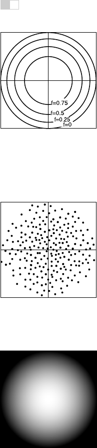
Figure 28.1. A contour
plot for four levels of the
function 1 - x
2
-y
2
.
For simplicity, assume that our 2D scalar data is defined as
f(x, y)=
1 − x
2
− y
2
, if x
2
+ y
2
< 1,
0 otherwise,
(28.1)
over the square (x, y) ∈ [−1, 1]
2
. In practice, we often have a sampled represen-
tation on a rectilinear grid that we interpolate to get a continuous field. We will
ignore that issue in 2D for simplicity.
One way to visualize a 2D field is to draw lines at a finite set of values
f(x, y)=f
i
(shown for the function in Equation 28.1 in Figure 28.1). This
is done on many topographic maps to indicate elevation. Isocontours are excel-
lent at communicating slope, but are hard to read “globally” to understand large
trends and extrema in the data.
Another common way to visualize 2D data is to use small pseudorandom dots
whose density is proportional to the value of the function. This is shown for our
test function in Figure 28.2. Such random density plots are useful for display on
black-and-white media, but are otherwise usually not a good choice for visualiza-
tion. Random density plots look smoother and smoother as more and smaller dots
are used maintaining overall density. As the dot size shrinks below human visual
Figure 28.2. A random
density plot for four levels of
the function 1 - x
2
-y
2
.
acuity, the image looks smooth. This results in a grayscale continuous tone plot
of the function. It is hard for humans to read such plots, because our ability to
detect absolute intensity levels is poor. For this reason, color or thresholding is
often used. This is shown in grayscale in Figure 28.3. Formally, we can specify
such a mapping with just a function g that maps scalar values to colors:
g : R → [0, 1]
3
.
Here [0, 1]
3
refers to the RGB cube. A common strategy is to specify a set of
colors to which specific values map and linearly interpolate colors between them.
A set of colors that increases in intensity and cycles in hue is often used. Such a
set of colors for the domain [0, 1] is
Figure 28.3. A grayscale
density plot of the function
1-x
2
-y
2
.
g(0.00) = (0.0, 0.0, 0.0)
g(0.25) = (0.0, 0.0, 1.0)
g(0.50) = (1.0, 0.0, 0.0)
g(0.75) = (1.0, 1.0, 0.0)
g(1.00) = (1.0, 1.0, 1.0)
Get Fundamentals of Computer Graphics, 3rd Edition now with the O’Reilly learning platform.
O’Reilly members experience books, live events, courses curated by job role, and more from O’Reilly and nearly 200 top publishers.

