Excel Annoyances

PIVOTTABLE ANNOYANCES

LEARN TO USE PIVOTTABLES

The Annoyance:

I’ve heard Excel aces talk about PivotTables as if they were some great gift to spreadsheet users. Then, the owner of a chain of local pet stores asked me in a job interview if I knew how to make and manipulate the darned things. I didn’t know and, rather than lie, I told him no, but that I was willing to learn. He hired me, but if I want to get past my probation period, I’m gonna have to learn how to use them. So, I ask: what the heck is a PivotTable, and how do I create one?

The Fix:

A PivotTable is a dynamic data table (sort of a report, actually) that you can manipulate to emphasize different views of a data list stored in Excel. As an example, consider the worksheet shown in Figure 4-24.

Figure 4-25. This configuration emphasizes days over hours.

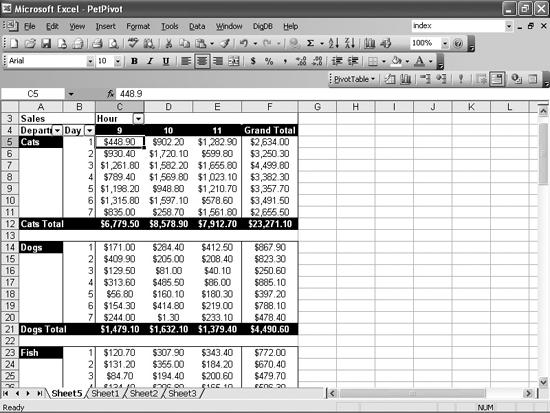
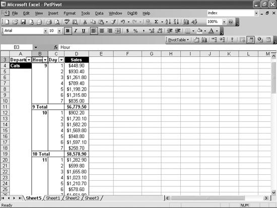
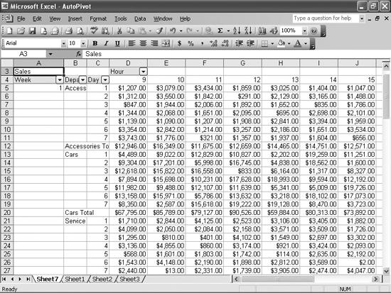
This PivotTable shows a sampling of the hourly sales for the departments in your boss’s four pet stores. The rows are grouped by department and then by day, while each column represents an hour of the day. You could produce exactly the same worksheet without using the PivotTable feature, but then you wouldn’t be able to change it without rearranging all the data by hand to produce a different look, such as the one shown in Figure 4-25.

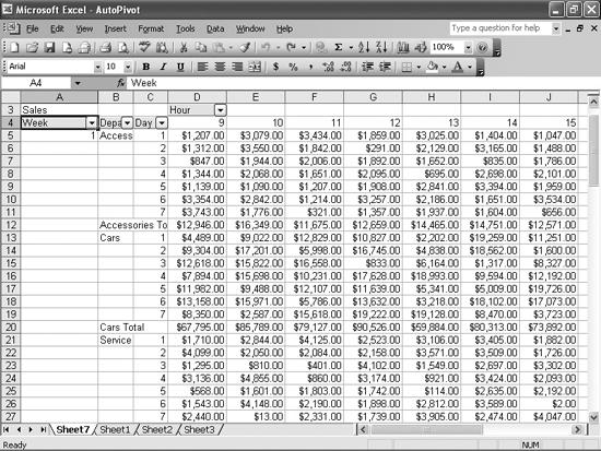
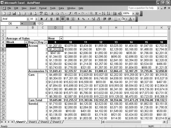
The PivotTable configuration in Figure 4-25 shows each department’s sales, but instead of arranging it by day, it emphasizes sales during specific hours of the day (9:00 AM, 10:00 AM, and so on). That’s the power of the PivotTable: you can change from one data arrangement to another quickly, perhaps as part of a presentation, and show how your sales break down by department, week, day, or even hour.

Figure 4-26. This configuration emphasizes hours over days.

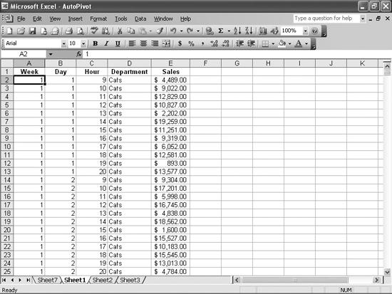
To create a PivotTable, your data needs to be arranged as a list, as shown in Figure 4-26. The order of the columns isn’t important, but it’s easier to read your data if you arrange the columns in a logical order.

Figure 4-27. This data is ready to be made into a PivotTable.

Although the order of your columns doesn’t matter, your data list must follow a few rules before Excel can use it to create a PivotTable:

• There can be no blank rows and no blank columns in the list.

• Each column must have a unique name.

• There should be no extraneous data in cells neighboring the list. That means you must have either the left edge of the worksheet or a blank column adjoining the list on either side, and you need at least one blank row at the bottom.

• There can be no duplicate keys.

Please note that each row denotes a unique bit of information. As an example, consider the data in row 2 of Figure 4-26 (the row just below the column headers). This row provides the sales total for the Week (1), the Day (1), the Hour (9), and the Department (Cats). The next row provides the sales total for the Week (1), the Day (1), the Hour (10), the Department (Cats), and so on, row by row. Each row in the data list corresponds to a cell in the Pivot-Table.

It’s absolutely vital that each row provides a unique data point. In this example, the first four columns (Week, Day, Hour, and Department) combine to form a unique value, or key, for each row in the column. It wouldn’t make any sense to have the two rows shown in Figure 4-27.

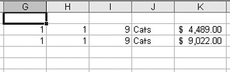
Figure 4-28. These rows compete to see which value is used in the PivotTable. It’s a fight no one will win.

Those rows attempt to set a different value for sales on Week: 1, Day: 1, Hour: 9, and Department: Cats, and it’s the sort of error that will bring the PivotTable Wizard to a screeching halt. The Sales column, which provides the data displayed in the body of the PivotTable, doesn’t matter...Excel wouldn’t care if every value in the Sales column were the same. What you can’t have are two or more rows in the list where the nondata fields are an exact match.

CREATE A PIVOTTABLE

The Annoyance:

OK, I followed all those complicated rules and I thought my data list was ready to make into a PivotTable. So, I chose Data → PivotTable Report in Excel 97 and tried to work my way through the PivotTable Wizard, but I didn’t understand some of the questions, and Excel didn’t seem to recognize the data list I wanted to use. Help!

The Fix:

To create a PivotTable in Excel 97, follow these steps:

1. Select any cell in your data list and choose Data → PivotTable Report.

2. Select the “Microsoft Excel list or database” option and click Next.

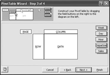
3. Verify that the proper data range appears in the Range field and click the Next button to display the third page of the PivotTable Report Wizard, as shown in Figure 4-28. (If the data range in the Range field is not correct, click the Collapse Dialog button next to the Range field. Then select the cells from your worksheet, click the Expand Dialog button at the right of the field, and click the Next button to display the third page of the PivotTable Report Wizard.)

4. Drag the field headers to the desired positions in the PivotTable. The order of the field headers determines how Excel will group the PivotTable’s data. To duplicate the layout seen in Figure 4-29, drag the Week, Department, and Day fields (in that order) to the Row area, the Hour field to the Column area, and the Sales field to the Data area. Click Next when you’re done.

5. Verify that the New Worksheet option is selected and click Finish.

Figure 4-29. Create the initial layout of your PivotTable here.

To create a PivotTable in Excel 2000, 2002, or 2003, follow these steps:

1. Select any cell in your data list and choose Data → PivotTable and PivotChart Report.

2. Select the “Microsoft Excel list or database” option, and then the PivotTable option, and click Next.

3. Verify that the proper data range appears in the Range field, click Next, and then click the Layout button.

4. Drag the field headers to the desired positions in the PivotTable. The order of the field headers determines how Excel will group the PivotTable’s data. To duplicate the layout seen in Figure 4-29, drag the Week, Department, and Day fields (in that order) to the Row area, the Hour field to the Column area, and the Sales field to the Data area. When you’re done, click OK.

5. Make sure “New worksheet” is selected, and click Finish.

Tip

You can find out how to create PivotCharts in Chapter 5.

PIVOT A PIVOTTABLE

The Annoyance:

I created a PivotTable, and it looks pretty good in its base configuration (shown in Figure 4-29), but I guess I missed the meeting in which they described how to rearrange my data on the fly. How do I change its groupings to emphasize other aspects of the data?

Figure 4-30. This is only one way to look at your PivotTable data.

The Fix:

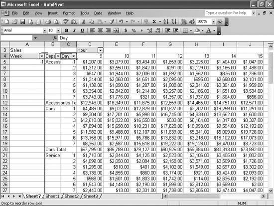
To pivot a PivotTable, choose Data → PivotTable Report (or Data → PivotTable and PivotChart Report, depending on your version), and drag a field header to the new position in the PivotTable. When you drag the field header over the row, column, or page area, you’ll see a gray I-bar appear, as in Figure 4-30. When you release the left mouse button, Excel regroups the PivotTable data.

Figure 4-31. The gray bar tells you where your PivotTable header will end up when you release the left mouse button.

FILTER PIVOTTABLE DATA

The Annoyance:

My PivotTable contains much more data than will fit on one screen. I see what appear to be filter arrows at the right edge of each field header. Can I use them to limit the data that appears in my PivotTable?

The Fix:

To filter a PivotTable in Excel 2000 and later, click the filter arrow at the right edge of a field header and select the values you want to appear. If the Show All box at the top of the list is checked, unchecking it deselects all the values in the list; if the Show All box isn’t checked, checking it selects every item in the list.

To filter an Excel 97 PivotTable, double-click a field header to display the PivotTable Field dialog box (shown in Figure 4-31). Select the values you want to hide in the Hide Items drop-down list, and click OK. To redisplay the items double-click the field header and deselect the items.

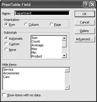
Figure 4-32. PivotTables are based on data lists. Just as you can filter a list, you can filter a PivotTable.

Filtering the data in your PivotTable won’t affect the source data.

CREATE ADVANCED PIVOTTABLE FILTERS

The Annoyance:

I created a PivotTable, and I want to emphasize certain aspects of the data, such as the top 10 (or bottom 10) sales days for my auto dealership’s service department. I know how to do it using an AutoFilter in a regular data list; is there a way to do it in a PivotTable?

The Fix:

Starting with Excel 97, you can use the equivalent of the AutoFilter Top 10 feature to display the top or bottom values in your PivotTable’s data field. The specific method you use to activate the filter has changed as PivotTables have evolved, but it’s there if you know where to look. For the purposes of this fix, assume you’re using the PivotTable in Figure 4-32.

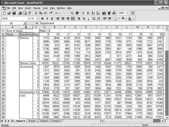
Figure 4-33. It’s possible to find the top or bottom values in a PivotTable, but how you do it depends on the version of Excel that you’re using.

To display a number of top or bottom values in an Excel 97 or 2000 PivotTable, follow these steps:

1. Click any cell in the PivotTable and choose Data → PivotTable Report (that’s Data → PivotTable or PivotChart Report in Excel 2000).

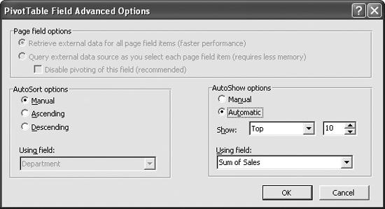
2. Double-click the row or column field header you want to use to find the top or bottom subset of data. The PivotTable Field dialog box appears. Click Advanced to display the PivotTable Field Advanced Options dialog box (shown in Figure 4-33).

   

   Figure 4-34. These advanced options include filtering your data.

3. Select the Automatic option.

4. Select Top or Bottom from the Show pull-down list, and specify the number of items to display in the field just to the right.

This same technique I just explained for Excel 97 and 2000 works perfectly well in Excel 2002 and 2003, but there’s a faster way to invoke the top/bottom 10 feature in these later versions of the program:

1. Click any cell in the field by which you want to sort. For example, if you wanted to sort the PivotTable in Figure 4-32 by day, you could click cell C5 (or C6:11, etc.).

2. If necessary, right-click a blank spot on any toolbar and choose PivotTable to display the PivotTable toolbar.

3. Choose PivotTable → Sort and Top 10.

4. Select the On option, and use the Show field to set the number of values at the top or bottom of the list to display.

FILTER A PIVOTTABLE BY ANY FIELD

The Annoyance:

I created a PivotTable with all the fields I wanted to use to group and filter my data, but now I’d like to filter my PivotTable using values from a field I didn’t use in the grouping. For example, I’d like to create a PivotTable, such as the one in Figure 4-34, that doesn’t use the Week field values to group the data, but I’d still like to be able to use the Week field to limit the data shown in the PivotTable. Is there a way to do that?

Figure 4-35. You don’t need to sort your data by week, but you might need to filter it by week. No problem.

The Fix:

To filter a PivotTable using a field that isn’t used to group the PivotTable data, move the field header to the Page area in the PivotTable layout box, as shown in Figure 4-35.

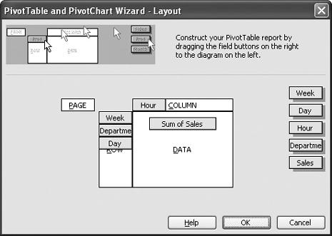
Figure 4-36. The Page area is your repository for fields you want to use just to filter your PivotTable data.

To display the layout box in Excel 97, click any cell in the PivotTable and choose Data → PivotTable Report. In Excel 2000 and later choose Data → PivotTable and PivotChart Report → Layout. In Excel 2000 and later, you also can drag a field header to the Drop Page Fields Here area of the PivotTable report. Once the field header is in the Page area, you can filter the PivotTable as if the header were in the Row or Column area.

FIND PIVOTTABLE ADD-INS

The Annoyance:

I like using PivotTables, but I don’t have time to learn how to do everything. Are any add-ins available that can help me do things such as set the print area, freeze the rows at the top of the Pivot-Table, and so on?

The Fix:

The following add-ins are available:

• PivotTable AutoFormat XL records and applies custom formats for your PivotTables. You can download it from http://www.ablebits.com/excel-pivottables-autoformatting-addins/, for $39.95.

• PivotTable Helper is a free add-in for Excel 2000 and later that extends the capabilities of the PivotTable Auto-Format XL add-in. It adds buttons to the AutoFormat toolbar that enable you to quickly perform tasks such as selecting an entire PivotTable, changing the number of decimal places displayed in the data area, and adding or removing Grand Total rows. Download it from http://www.ablebits.com/excel-pivottables-formatting-assistant-free-addins/index.php.

• With PivotTable Assistant, you can resize columns for easier viewing, set the print titles and area for printing out a PivotTable, freeze title rows and columns for easy viewing, and add borders to the bottom and right side of each printed page of a PivotTable. It’s available at http://www.ozgrid.com/Services/Excel-pivot-table-assistant.htm for $29.95.

APPLY AUTOFORMAT TO A PIVOTTABLE

The Annoyance:

My PivotTables look great, but when I try to add formatting, such as displaying a value in boldface or italic, and then pivot the table, the cell formats don’t pivot with the values. They stay in place, which means they are applied to the wrong cells. I know you can apply an AutoFormat to a table in an Excel worksheet. Is there a way to apply an AutoFormat to a PivotTable?

The Fix:

To apply an AutoFormat to a PivotTable, click any cell in the PivotTable, choose Format → AutoFormat, and select the AutoFormat you want to apply. If you want to create your own PivotTable AutoFormats, you can use the Pivot Table AutoFormat XL add-in discussed previously.

STOP PIVOTTABLES FROM PIVOTING!

The Annoyance:

I created several PivotTables in Microsoft Excel 2000 to analyze sales data, but changes I make to one PivotTable seem to affect the others I’ve created from the same data. What’s going on?

The Fix:

The problem is that you followed Excel’s advice when you created the second (and subsequent) PivotTables based on the same data. When you create a second PivotTable from the same data source, Excel displays the advisory message Your new PivotTable will use less memory if you base it on your existing PivotTable [Work-bookName]SheetName!PivotTableName, which was created from the same source data. Do you want your new PivotTable to be based on the same data as your existing PivotTable? It seems like a reasonable thing to do, but it is, in fact, a very bad idea.

When you create a PivotTable, Excel creates a cache that contains the data and structure (that is, field groupings) for the PivotTable. When you use one PivotTable as the data source for a second PivotTable, any changes to any of those PivotTables that share the same memory cache will affect all the other PivotTables. You can avoid this behavior by clicking No when Excel asks if you want to base your PivotTable on the same data as an existing Pivot-Table. Then Excel will create a separate memory cache for the new PivotTable, and your PivotTables will pivot independently.

PIVOTTABLE DATA DISPLAYS AS NUMBER SIGNS

The Annoyance:

I don’t have a huge data list, so I created my PivotTable on the same worksheet as the original data. The problem is that Excel now displays some of my source data as number signs (#####). What’s going on, and how do I fix it?

The Fix:

What’s happening is that Excel is reformatting the width of your worksheet columns to fit the contents of your PivotTable—and if there’s no room in a cell to display the source data, Excel uses number signs. You can prevent Excel from changing your columns’ widths by turning off the Autoformat Table option in the PivotTable Wizard. The procedure you follow depends on your version of Excel.

To turn off the Autoformat Table option in Excel 97, follow these steps:

1. Select a cell contained in your PivotTable and choose Data → PivotTable Report.

2. Click Next to get to the fourth step of the PivotTable Wizard, click the Options button, and uncheck the “Autoformat table” box.

In Excel 2000, follow these steps:

1. Select a cell contained in your PivotTable and choose Data → PivotTable and PivotChart Report.

2. Click Next twice to advance to page 3 of the PivotTable and PivotChart Wizard.

3. Click Options, and then uncheck the “AutoFormat table” box.

In Excel 2002 and 2003, right-click any cell in the PivotTable, choose Table Options, and uncheck the AutoFormat table box.

“PIVOTTABLE IS NOT VALID” ERROR

The Annoyance:

I support a large mail order retail sales firm where the IT folks get the fancy software and we get very old versions of Office. I was so frustrated I brought in my own, unopened copy of Office 2000, but I’m the only person in my section that has anything that recent—everyone else uses Office 97. I created a PivotTable from something called an OLAP (Online Analytical Processing) cube in Excel 2000, went to our meeting room (which has a PC running Excel 97), and tried to use the PivotTable in a presentation. I got a “PivotTable is not valid” error message. Because I couldn’t find the “Yes, it is!” button, I ended up having to wave my hands instead of doing the cool stuff I had planned. What happened?

Online Analytical Processing

Online Analytical Processing (OLAP) is technology that makes large collections of data easier to analyze and present by summarizing and arranging the data in response to user queries—and if you’re using it, you probably know what you’re doing. Excel PivotTables can handle the data summaries, but would choke on the massive database tables generated by most large business systems.

The Fix:

As you probably guessed, Excel 97 simply can’t handle PivotTables based on data in OLAP cubes. That functionality wasn’t introduced until Excel 2000. Excel 97 will display the PivotTable in the state in which it was saved in Excel 2000, but you can’t pivot it or refresh its data. You can work around this problem in two ways. The first workaround is to create a new PivotTable for each configuration you want to display on the Excel 97 computer. I recommend putting the PivotTables in separate worksheets and renaming the worksheets to reflect the emphasis of each PivotTable. The other workaround is to import the OLAP data into an Excel 2000 workbook, open the workbook in Excel 97, and create a new PivotTable.

PIVOTTABLE LOSES FORMATTING

The Annoyance:

When I created the worksheet I use to track sales, I formatted the numbers in the Currency style, but when I create a PivotTable from that data, Excel loses the formatting. Is there any way I can retain data formatting when I create the PivotTable, or at least add the formatting quickly afterward?

The Fix:

It’s a sad fact of life that you lose your data field’s formatting when you create a PivotTable. Microsoft Knowledge Base article #214021 offers a fix—you’re supposed to click Options on the next-to-last (Excel 97 and 2000) or last (Excel 2002 and 2003) PivotTable Wizard page, and check the Preserve Formatting checkbox—but it didn’t work for me in any version of Excel. What I can tell you is that there’s a quick way to format your data in every version since Excel 97. To format the data field of a PivotTable quickly, right-click any cell in the data area and choose Field (Excel 97 and 2000) or Field Settings (Excel 2002 and 2003) to display the PivotTable Field dialog box (shown in Figure 4-36).

Figure 4-37. Here’s where you go to find the Format Cells dialog box for your PivotTable.

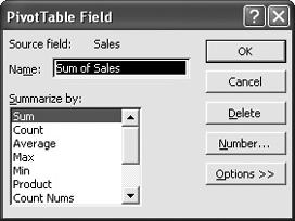
Once in the PivotTable Field dialog box, click the Number button and use the Number page of the Format Cells dialog box to define your data’s format.

USE CALCULATED FIELDS IN A PIVOTTABLE

The Annoyance:

PivotTables are fine as far as they go, but I’d like to do more with the data in the table. For example, 3% of my company’s revenue goes to a corporate overhead fund that pays the light bill, office supplies, and environmental cleanup for antifreeze spills. I’d like to have a field riding alongside the body of the PivotTable (as shown in Figure 4-37) that lists the overhead deduction associated with the data in the table. Is there any way to do that?

Figure 4-38. This PivotTable answers your questions.

The Fix:

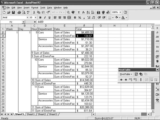
Excel 97 introduced the calculated field (a user-defined field that derives its value from a formula you create) and the calculated item (a user-defined field that derives its value from a particular entry in a column—e.g., the “Cars” entry in the Department column). For example, if you wanted to determine the amount of the 3% overhead fund deduction from hourly sales, you could create a calculated field with the formula =Sales * .03 to display the amount.

To add a calculated field to a PivotTable, follow these steps:

1. If it isn’t already on, turn on the PivotTable toolbar by selecting View → Toolbars.

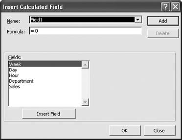
2. Select any cell in the PivotTable, and then, on the PivotTable toolbar, choose PivotTable → Formulas → Calculated Field to display the Insert Calculated Field dialog box, shown in Figure 4-38.

   

   Figure 4-39. Create additional fields based on any formula you want.

3. Type the name of the calculated field in the Name field, type your formula (such as =Sales * .03) in the Formula field, click the Add button, and then click OK.

4. The calculated field appears in the PivotTable data area.

To delete a calculated field, follow these steps:

1. Display the PivotTable toolbar.

2. Choose PivotTable → Formulas → Calculated Field to display the Insert Calculated Field dialog box.

3. Open the Name drop down, select the calculated field you want to whack, click Delete, and then click OK.

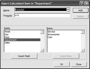
Creating a calculated item is similar to creating a calculated field, except you need to decide at which grouping level to create the calculated item. For example, in the PivotTable shown in Figure 4-37 you could create a calculated item named NonCarSales that added sales from the Accessories and Service categories and included those results in the body of the PivotTable. You would need to create the formula using the format =Column[Value1] + Column[Value2] so that Excel can identify which elements you want to calculate. For example, the formula to add Accessories and Service sales would be =Department[Accessories] + Department[Service] .

To add a calculated item to a PivotTable, follow these steps:

1. Click the field header that corresponds to the field you want to use in your calculations (in this case, click Department).

2. On the PivotTable toolbar, choose PivotTable → Formulas → Calculated Item to display the Insert Calculated Item dialog box, shown in Figure 4-39.

   

   Figure 4-40. You also can create fields that pivot along with the rest of your PivotTable data.

3. Type a name for the calculated item in the Name field, type the formula for the calculation in the Formula field, and then click Add.

PIVOTTABLES WITH SUPERPOWERS

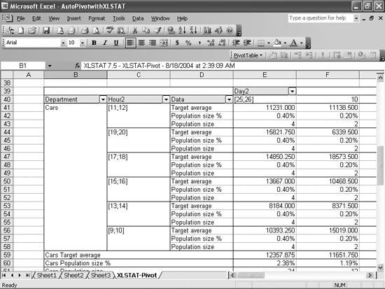
I thought I was pretty good with PivotTables until I saw what the XLSTAT-Pivot add-in from Addinsoft can do. It’s a powerful program that helps you quantify the effect that different variables, such as the hour of the day or the day of the week, have on your business. The PivotTables you can create using XLSTAT-Pivot (shown in the following figure) are mind-blowing. You can have the program look at how closely variables are correlated, chart the percentage contribution each variable makes to your business, and determine the likelihood that the data model is correct by using measures of robustness.

There’s only one catch. Well, two catches. OK, actually, there are three. First, XLSTAT-Pivot requires Excel 2000 or later, which is no biggie. Next, it requires you to have already installed XLSTAT-Pro.

The third catch is the big one: between them, these two applications run a cool $1,385 ($395 for XLSTAT-Pro, $990 for XLSTAT-Pivot). The good news is that you can download 30-day trial versions of both programs from the company’s site at http://www.xlstat.com/, so you’ll get a chance to try before you buy. You also can run through the XLSTAT-Pivot tutorial at http://www.xlstat.com/demo-pivot.htm, which gives you a good idea of how the program works.

The trial versions you download are executable files, so all you need to do is double-click the files to install the programs. When it comes to trying out XLSTAT-Pivot, my advice is to print out the tutorial and walk through the procedure to check your progress. XLSTAT-Pivot is a tool for hard-core analysts who aren’t afraid to get their hands dirty; that’s for sure.

Figure 4-41. If you’re serious about analyzing your data using high-powered tools, consider adding XLSTAT-Pivot to your arsenal.

CHANGE SUMMARY CALCULATIONS IN A PIVOTTABLE

The Annoyance:

I used a PivotTable in a presentation the other day, and one of my company’s senior partners asked if there was any way to change how the PivotTable data is summarized. Specifically, she asked if I could display average sales instead of total sales in a Pivot-Table. Is there any way to change how Excel summarizes PivotTable data?

The Fix:

You can, in fact, change the summary operation Excel uses in a PivotTable. To do so, right-click any cell in the PivotTable’s data area and choose Field to display the PivotTable Field dialog box (shown in Figure 4-40).

Figure 4-42. Sums and totals aren’t your only options when summarizing PivotTable data.

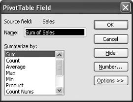
Select the summary calculation you want to use from the drop-down list, and click OK to apply it to the PivotTable. For example, if you wanted to find the average hourly sales over a week, you would select Average. When you click OK, you’ll see the PivotTable shown in Figure 4-41.

Figure 4-43. Here’s where you find what you can do with your summaries.

HIDDEN DATA DOESN’T APPEAR IN THE SUMMARY

The Annoyance:

My boss uses the PivotTables I create to show how much each department contributes on a daily and weekly basis to our bottom-line profits. One thing he doesn’t like, however, is that Excel doesn’t display a “filtered” total for a column when you filter it—it displays only the total for the visible values (as shown in Figure 4-42). Is there any way to have Excel display the total for all items, both visible and hidden?

Figure 4-44. You control whether a PivotTable bases its calculations on all the values, or just the visible ones.

The Fix:

To have Excel include hidden values in its subtotals, right-click any cell in the PivotTable’s data area, choose Table Options (Options in Excel 97), and place a check in the “Subtotal hidden page items” checkbox.

“REFERENCE NOT VALID” ERROR

The Annoyance:

I used a data form to enter the values for my PivotTable’s data list, but now when I try to create a PivotTable based on that data, I get an error message saying “Reference is not valid.” I know the reference is valid—it’s just a data list, like dozens of data lists I’ve used before. Sheesh! One thing I did notice is that for some reason Excel is displaying the reference Database in the second page of the PivotTable Wizard (see Figure 4-43). I can select the range before I run the Wizard, but I’d rather let Excel detect the data list automatically. What’s going on?

Figure 4-45. The data list looks like it should work, and it should—except for one detail.

The Fix:

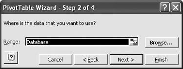
The problem is that when you create a data entry form to enter data into a list, Excel creates a named range called Database. What’s worse, the Database named range is invisible, and doesn’t show up in the Define Name dialog box. To delete the Database named range, follow these steps:

1. Select any cell in the worksheet and choose Insert → Name → Define to display the Define Name dialog box.

2. In the “Names in workbook” field, type Database.

3. Click Add, and then click Delete.

Excel will now detect the data list in the usual manner.

DISPLAY PIVOTTABLE DATA AS A PERCENTAGE OF A TOTAL

The Annoyance:

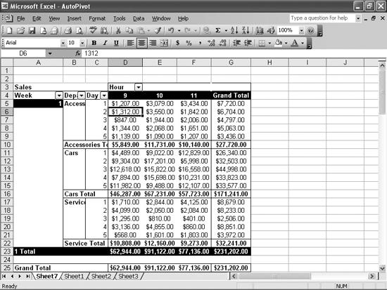
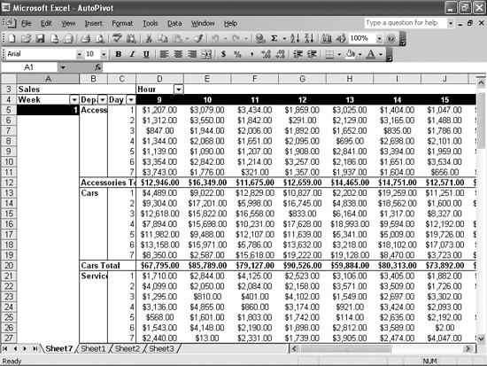
I’d like to display my sales data as a percentage of a total, not just as a value with a running total in the far-right column of my PivotTable. For example, assuming the data in Figure 4-44, how can I display each day and hour as a percentage of a column and how do I change the display so that I see percentages of days and weeks instead of a percentage of the entire column?

Figure 4-46. If you can’t figure percentages in your head, you’ll need to change how Excel dislplays this data.

The Fix:

To display the values in an Excel 97 PivotTable as a percentage of a column total, follow these steps:

1. Click any cell in the PivotTable and choose Data → PivotTable Report.

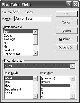
2. On the third page of the PivotTable Wizard, double-click Sum of Sales and then, in the PivotTable Field dialog box, click the Options button (the result is shown in Figure 4-45).

   

   Figure 4-47. Use the controls in this dialog box to change how Excel summarizes your PivotTable data.

3. Click the down arrow at the right of the “Show data as” field and choose “% of Column” from the drop-down list.

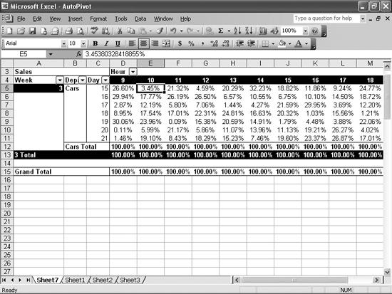
In Excel 2000 and later, double-click the Sum of Sales field header in the body of the PivotTable to display the PivotTable Field dialog box and follow the same procedure. Then you can filter the data in the PivotTable, which will cause Excel to update the percentage calculations (as shown in Figure 4-46).

Figure 4-48. The end result answers your questions.

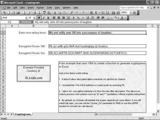
CRYPTOGRAM GAME

If you like the CryptoQuote decryption game in the newspaper, you’ll enjoy Aaron Blood’s free cryptogram generator, which you can download from http://www.xl-logic.com/xl_files/games/cryptogram.zip. You have to enter the text to be encrypted, as shown in the following figure, but you can have a group of friends rotate who generates the next cryptogram so that everyone gets a chance to play. If you want to be really sneaky, misspell one of the words. Drives people crazy.

Figure 4-49. Cryptograms are a fun single substitution for work.