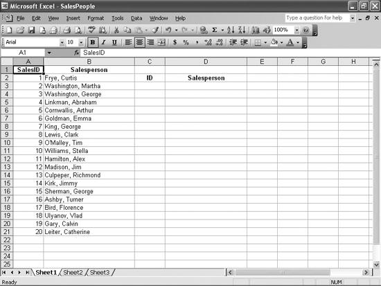
I know Excel isnât a database...thatâs Access. And I know I shouldnât expect miracles, but Iâm hoping you can help me look up a value in a table. For example, I have a list of sales reps, sorted by their employee ID number (as in Figure 4-8). If I see a transaction report with an employee ID, isnât there some way I can look up who belongs to that number without using the Find function?
Sure, you can do it. The process involves some pretty fancy footwork with advanced Excel functions, but once you grasp whatâs going on youâll be fine.
The first function you can use to find a value in a worksheet is the
LOOKUP()
function. Basically, the
LOOKUP()
function identifies a row in your worksheet by looking in, say, column A for a value you specify. Once it identifies the row that contains that value in column A, it looks in, say, column C of that same row, snatches the value it finds there, and âreturnsâ it, or displays it, in whatever cell holds your formula.
The
LOOKUP()
function has this syntax:
=LOOKUP(lookup_value, lookup_vector, result_vector)whereby:
lookup_value is the cell (or value) to find in the table. It could be an employeeâs ID number, a Social Security number, or another unique identifier.
lookup_vector is the range to search for the lookup_value . If a list of employee IDs were stored in the range A2:A34, you would type A2:A34 in the lookup_vector spot.
result_vector is the range within which to look, find, and return the corresponding value. If the employeesâ names are stored in the range B2:B34, thatâs the range youâd type here.
In other words, youâre telling the
LOOKUP()
function what to look for, where to look for it, and where to find the corresponding value youâre really interested in. In the worksheet in Figure 4-8, if you enter the formula
=LOOKUP(C3,A2:A21,B2:B21)
into a blank cell, it will take the value you enter into C3, locate the matching value in column A (looking from row 2 to 21), and return the value in column B that corresponds with the value found in column A. Typing 5 in cell C3 would return Cornwallis, Arthur, while typing 16 in cell C3 would return Ashby, Turner.
The
LOOKUP()
function is somewhat limited in that the
lookup_vector
and
result_vector
can consist of only one row or column each. Thereâs also the possibility of getting an incorrect result: if
LOOKUP()
canât find the
lookup_value
in the
lookup_vector
table, it matches the largest value that is less than or equal to
lookup_value
. In the case of the worksheet in Figure 4-8, if you hired a new sales rep who was assigned SalesID 21, but you didnât enter the repâs information into the worksheet, searching for the value would return Leiter, Catherine, which is incorrect.
If you donât mind going to a little more trouble, you can avoid bogus matches and go beyond the two-column limit by using the
VLOOKUP()
function instead. The
VLOOKUP()
function has the following syntax:
=VLOOKUP(lookup_value, table_array, col_index_num, range_lookup)whereby:
lookup_value is the value to be found; it can be a value (the number 14), a reference to a cell where the value appears (cell D2), or a text string (the part identification code GR083).
VLOOKUPalways looks for thelookup_valuein the first column of the array.table_array is the cell range in which Excel should search for the lookup_value . The table_array in Figure 4-8 is the range A2:B21.
col_index_num is the column number in table_array in which the matching value will be found and returned. A col_index_num of 1 returns the value found in the leftmost column in table_array , a col_index_num of 2 returns the value found in the second column in table_array , and so on. If col_index_num is greater than the number of columns in the range named in the table_array argument,
VLOOKUP()displays a #N/A error code.range_lookup is an optional argument. When set to TRUE or left blank,
VLOOKUP()works like theLOOKUP()function and returns the largest value that is less than the lookup_value . If set to FALSE, the function must find an exact match or it will display an #N/A error code.
The
VLOOKUP()
function thatâs equivalent to the
=LOOKUP(C3,A2:A21,B2:B21)
formula I discussed earlier is
=VLOOKUP(C3,A2:B21,2,TRUE)
.
Incidentally,
VLOOKUP()
doesnât distinguish between uppercase and lowercase text. If you need to create a lookup function that distinguishes between uppercase and lowercase, see the annoyance "Perform a Case-Sensitive Lookup" later in this chapter.
The
VLOOKUP()
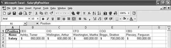
function is short for vertical lookup, which means Excel assumes your data is arranged in columns. If your data happens to be arranged in rows, as is the case in Figure 4-9, you can use the
HLOOKUP()
function to search for corresponding values.
The
HLOOKUP()
function uses this syntax:
=HLOOKUP(lookup_value, table_array, row_index_num, range_lookup)And it works exactly the way
VLOOKUP()
does, except at right angles:
lookup_value is the value to be found in the first row of the table.
table_array is the cell range to be searched.
row_index_num is the row number in table_array from which the matching value will be found and displayed as the formulaâs result. In other words, if your worksheet had a series of employee IDs in the first row, the employeesâ names in the second row, and the employeesâ salaries in the third row, a row_index_num value of 2 would find a name, while a row_index_num value of 3 would find the salary. If row_index_num is less than 1,
HLOOKUP()returns a #VALUE! error; if row_index_num is greater than the number of rows in table_array ,HLOOKUP()returns a #REF! error.range_lookup , if set to TRUE or omitted, allows
HLOOKUP()to find an approximate match. If set to FALSE,HLOOKUP()must either find an exact match or display an #N/A error.
For this table, the formula to look up the salary associated with the position (CEO, CIO, COO, etc.) entered into cell B12 would be
=HLOOKUP(B12,B2:F3,3,FALSE)
.
The
VLOOKUP()
function is neat. But you canât use it to look up a value in any column except column A. That means if I want to look up a value in the fifth column and return the corresponding value from the third column, Iâm out of luck. Is there a way around this limitation of the
VLOOKUP()
function?
You can search for values in an arbitrary column and return a corresponding value from another column, but you need to use a combination of the
INDEX()
and
MATCH()
functions to do it. The
INDEX()
function, which finds the address of a cell that meets a criterion, has the following syntax:
    =INDEX(
                     reference, row_num, column_num, area_num
                  )
whereby:
reference is a reference to one or more cell ranges that contain the values you want the function to look for and return. If you want to search a noncontiguous group of cells, youâll need to enclose the references in parenthesesâe.g., (A1:B6, C3:D8, F1:G6).
row_num is the number of the row in the range named in the reference argument where you want the function to look for the value.
column_num is the number of the column in the range named in the reference argument where you want the function to look for the value.
area_num is the cell range named in the reference argument where you want the function to look for the value. The first area selected or entered is numbered 1, the second is 2, and so on. If area_num is omitted,
INDEX()uses area 1. For example, ifINDEX()searched the ranges A10:B14, C12:D16, and F14:G18, A10:B14 would be area 1, C12:D16 would be area 2, and F14:G18 would be area 3.
The
MATCH()
function, by contrast, returns the relative position of a value in a cell range. For example, if the target value were in the third cell down in a single-column range,
MATCH()
would return the value 3.
The
MATCH()
function has the following syntax:
    =MATCH(
                     lookup_value, lookup_array, match_type
                  )
whereby:
lookup_value is the search term you use to find the value you want in a table.
lookup_array is a contiguous range of cells that contains a set of lookup values.
match_type is the number -1, 0, or 1. If match_type is 1,
MATCH()finds the largest value that is less than or equal to lookup_value . If this argument is set to 1, the values in lookup_array must be sorted in ascending order. If match_type is 0,MATCH()finds the first exact match to lookup_value . If this argument is set to 0, the values in lookup_array can be in any order. If match_type is -1,MATCH()finds the smallest value that is greater than or equal to lookup_value . If match_type is set to -1, the values in lookup_array must be sorted in descending order. If you donât specify a value for the match_type argument, Excel assumes itâs 1.
The
INDEX()
and
MATCH()
functions work well together because the
MATCH()
function supplies the cell location that the
INDEX()
function needs to do its lookup. As an example, consider the data set in Figure 4-10.
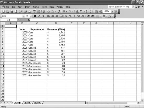
If you want to find the first instance when any department exceeded the $500,000 sales mark, first you would sort the sheet so that the Sales column is sorted in descending order, and then youâd use the formula
=INDEX(C3:C17,MATCH(F3,D3:D17,-1))
to find the department, and the formula
=INDEX(B3:B17,MATCH(F3,D3:D17,-1))
to determine the year when the sales mark was broken. Hereâs a rundown of what these compound formulas do:
The
INDEX()functionâs first argument defines the range with the potential values to be returned as C3:C17 (the auto dealershipâs departments).The
INDEX()function derives its second argument from theMATCH()function. TheMATCH()function uses the value in cell F3 to search the range D3:D17 for the smallest value that is larger than the value in F3; then it returns the cellâs position in the range (in this case, 5) to theINDEX()function.The
INDEX()function, which now looks like=INDEX(C3:C17,5), returns the value from cell C7, the fifth cell down in the sorted range.
I track my companyâs orders using an Excel 97 workbook that I converted from Lotus 1-2-3. I keep the orders on one worksheet and the actual products on another worksheet, but when I try to look up the product that corresponds to an order number, sometimes I get the wrong result. How come?
Excel 97 has a bug that rears its ugly head when your lookup table and the cell with the
VLOOKUP()
formula are on different worksheets, and you use the Transition Formula Evaluation option to have Excel resolve its formula as Lotus 1-2-3 would. (The two programs evaluate
VLOOKUP()
formulas differently.) To fix the problem, click the worksheet with the products lookup table, choose Tools â Options, click the Transition tab, and uncheck the âTransition formula evaluationâ checkbox.
I track the car and truck parts we stock at the auto dealership where I work. The part descriptions vary by manufacturer, of course, as do the codesâand many part codes, such as A3000 or T1648B, contain letters. Anyway, I just imported my list of part codes into Excel (see Figure 4-11) and was looking forward to using a manufacturerâs part code to look up the partâs name and other information, but when I tried I got an #N/A error. I typed A2000 instead of A3000 into the âsearch-forâ cell, so why did the formula generate an error? If I type in part number 9815 instead of 9816, the
VLOOKUP()
formula returns âSpark Plug,â which is the previous entry in the table. Why didnât the formula skip back to part number 9816, the entry before part A3000, and return âHeadlight?â Iâm totally confused.
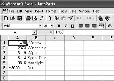
Excel doesnât react well when you mix text and numeric values in a lookup table. Excel tries to help you out by searching only for text values when you enter a text value, and only for numbers when you enter a number, but that can lead to problems. For instance, your sample worksheet contains a set of numeric values before the A3000 row, so the
VLOOKUP()
formula generates an error because the search made Excel try to go to a cell before the first text value.
The best way to prevent this error from occurring is to avoid mixing text and numeric values in a lookup list. If you canât do that, format the cells as text (select Format â Cells, click the Number tab, and select Text from the Category list) before you import or enter the data. If the data is already in the workbook, you can use an array formula to treat the values in the part code list as text (changing the formatting of the list cells after the data is entered wonât work). Hereâs the formula, which assumes the value you want to look up is in cell D2 and the part code list is in cells A1:A3:
{=VLOOKUP(TEXT(D2,"@"),TEXT(A1:A3,"@"),1)}Remember to press Ctrl-Shift-Enter to create this as an array formula; youâll get an #N/A error if you just press Enter.
I own a martial arts supply business, and Iâve run into a problem with one of my employees. Jo is a wonderful employee, but her name, when spelled in lowercase, happens to be the word for a type of stick we use around the dojo (and also a great word for Scrabble). When I try to use a lookup function to find a match for jo, sometimes I get a match for Jo. Thereâs gotta be a way to make a lookup function case-sensitive.
Well, if youâre doing just a simple search, you can require Excel to match the case of the search term by checking the âMatch caseâ checkbox in the Find dialog box (Edit â Find). If youâre planning to use one of the lookup functions (
HLOOKUP()
,
LOOKUP()
,
VLOOKUP()
,
INDEX()
, or
MATCH()
), there isnât an easy way to force them to require a case-sensitive match.
However, if you combine the IF() and EXACT() functions, you can make it happen. For example, assume youâre working with the worksheet shown in Figure 4-12.
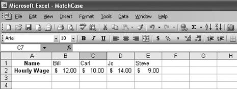
If you typed the formula
=IF(EXACT(B7,HLOOKUP(B7,A1:E2,1))=TRUE,HLOOKUP(B7,A1:E2,2),"No match")
into cell C7 and typed jo into cell B7, the formula would return No match because the lookup value in cell D1 is not in the same case as the entry in the table. However, if you typed Jo in cell B7, youâd see her hourly pay rate of $14.00.
The same technique works with a
LOOKUP()
formula, but you need to change the parameters a bit to match the
LOOKUP()
functionâs syntax. In this case, the data is arranged so that it can be used in a
LOOKUP()
function (as shown in Figure 4-13). In this case, the formula should be
=IF(EXACT(A7,LOOKUP(A7,A1:A5,A1:A5))=TRUE,LOOKUP(A7,A1:A5,B1:B5),"No match")
.
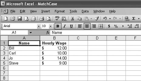
You also can use a
VLOOKUP()
formula with the data in Figure 4-13, which would be
=IF(EXACT(A7,VLOOKUP(A7,A1:B5,1,FALSE))=TRUE,VLOOKUP(A7,A1:B5,2,FALSE),"No match")
.
Iâm a marine biologist, and lately Iâve been studying the growth rate of a particular strain of bacteria in a fish habitat. I track the hourly growth rate in an Excel worksheet (shown in Figure 4-14), but occasionally Iâll get an error when I try to look up the values with a
VLOOKUP()
formula. Iâve never had any trouble with this function before, so why doesnât it like this particular data now?
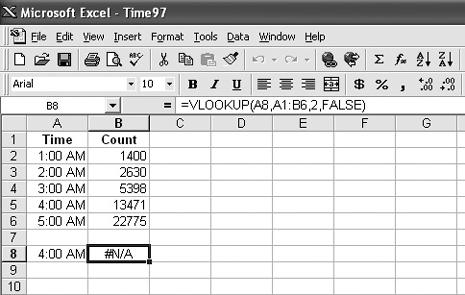
The problem, which occurs in every Excel version up to and including Excel 2003, kicks in when you use the fill handle to extend a sequence of times. In the worksheet shown in Figure 4-14, you probably typed 1:00 AM in cell A2, 2:00 AM in cell A3, and then extended the series using the fill handle into cells A4, A5, and A6. You can avoid the problem by entering the times manually, but thatâs not a good solution if more than three or four entries comprise a series. One possible solution is to choose Tools â Options, click the Calculation tab, and check the Precision as Displayed box. After you click OK, youâll see an error message that says Data will permanently lose accuracy, which applies to all the data in your workbook, not just in the current worksheet. In other words, if you have a set of numbers with five digits after the decimal, but youâve formatted the cells to display only the first two digits, Excel will truncate the actual values and forget the original cell value. If thatâs going to be a problem for you (and if youâre a scientist, it probably will), you need to keep your data as is (that is, with full precision), and if you want to use a
VLOOKUP()
formula that uses time values, you will need to enter all those time values by hand. Z-Z-z-z-z....
I maintain a master Excel 97 workbook that summarizes data from all the projects in my departmentâall 35 of them. I need to update the values in my summary workbook to keep up with new purchases and person-hours spent on the various projects, and yes, that does mean my workbook contains quite a few
VLOOKUP()
formulas that rely on importing data from other workbooks. The problem is that when I ask Excel to update those links and formulas, it takes forever (well, several minutes) for the workbook to open. These delays didnât happen in Excel 95! Is something broken?
The problem is that Excel has to open all the files youâre linked to before it can pull in the updated values. Excel 97, Excel 2000 (before Service Pack 1), and even Excel 2002 (before Service Pack 3) didnât handle opening the linked files well. The best way to get around the problem is to upgrade to Excel 2000 or 2002 and install the appropriate Service Packâor just bite the bullet and upgrade to 2003. You can download the most recent service pack for your version by visiting http://office.microsoft.com/OfficeUpdate/default.aspx. Click the Check for Updates link at the top of the page and the site will detect your version of Office and list the available downloads.
If you canât do any of those things for some reason, just make sure you open the files that youâve linked to before you update the values in your summary workbook.
I track orders from my customers in a database, and I import the data into an Excel worksheet so that I can create a PivotTable. The worksheet (shown in Figure 4-15) has the customerâs ID number in the first column and the order details in the next few columns. Whenever I use a
LOOKUP()
or
VLOOKUP()
formula to search the table, the formula finds the last occurrence in the table. Thatâs handy for finding the last time a customer placed an order, but what Iâd like to do is find the first time a customer placed an order. Is there a way to find the first occurrence of a value in a list instead of the last?

You can use a combination of the
INDEX()
and
MATCH()
functions to find the first occurrence of a value in a list. In the workbook shown in Figure 4-15, if the customer ID number 001354 were typed in cell D2, the formula
=LOOKUP(D2,A1:A6,B1:B6)
would return 1/5/2005, while the formula
=INDEX(A1:B6,MATCH(D2,A1:A6,0),2)
would return 10/15/2004. This particular combination of the
INDEX()
and
MATCH()
functions lets you perform the operation without sorting the listâs first column into either ascending or descending order.
Get Excel Annoyances now with the O’Reilly learning platform.
O’Reilly members experience books, live events, courses curated by job role, and more from O’Reilly and nearly 200 top publishers.

