Every Excel grandmaster needs to start somewhere. In this chapter, youâll learn how to create a basic spreadsheet. First, youâll find out how to move around Excelâs grid of cells, typing in numbers and text as you go. Next, youâll take a quick tour of the Excel ribbon, the tabbed toolbar of commands that sits above your spreadsheet. Youâll learn how to trigger the ribbon with a keyboard shortcut, and collapse it out of the way when you donât need it. Finally, youâll go to Excelâs backstage view, the file-management hub where you can save your work for posterity, open recent files, and tweak Excel options.
When you first fire up Excel, youâll see a welcome page where you can choose to open an existing Excel spreadsheet or create a new one (Figure 1-1).
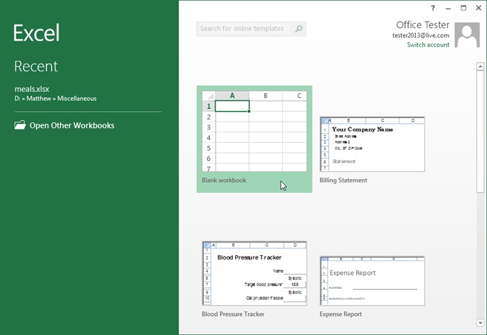
Figure 1-1. Excelâs welcome page lets you create a new, blank worksheet or a ready-made workbook from a template. For now, click the âBlank workbookâ picture to create a new spreadsheet with no formatting or data.
Excel fills most of the welcome page with templates, spreadsheet files preconfigured for a specific type of data. For example, if you want to create an expense report, you might choose Excelâs âTravel expense reportâ template as a starting point. Youâll learn lots more about templates in Chapter 16, but for now, just click âBlank workbookâ to start with a brand-spanking-new spreadsheet with no information in it.
Note
Workbook is Excel lingo for âspreadsheet.â Excel uses this term to emphasize the fact that a single workbook can contain multiple worksheets, each with its own grid of data. Youâll learn about this feature in Chapter 4, but for now, each workbook you create will have just a single worksheet of information.
You donât get to name your workbook when you first create it. That happens later, when you save your workbook (Saving Files). For now, you start with a blank canvas thatâs ready to receive your numerical insights.
When you click âBlank workbook,â Excel closes the welcome page and opens a new, blank worksheet, as shown in Figure 1-2. A worksheet is a grid of cells where you type in information and formulas. This grid takes up most of the Excel window. Itâs where youâll perform all your work, such as entering data, writing formulas, and reviewing the results.
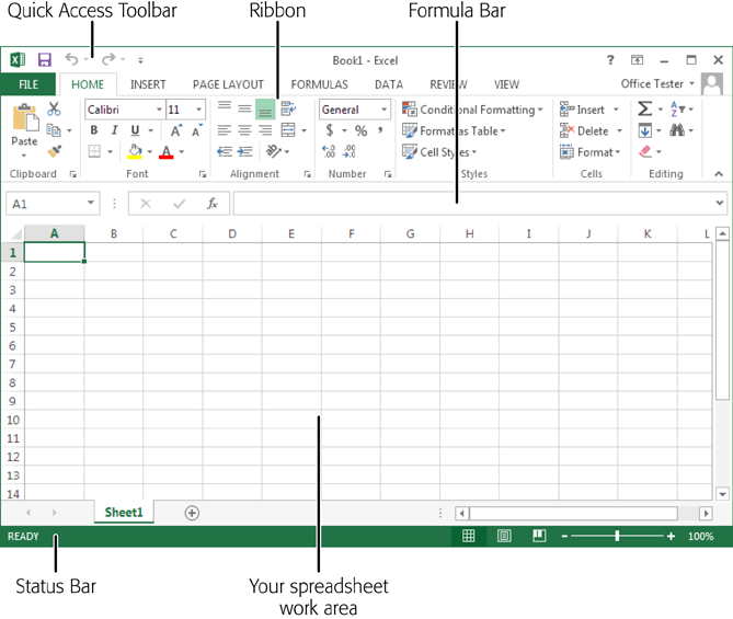
Figure 1-2. The largest part of the Excel window is the worksheet grid, where you type in your information.
Here are a few basics about Excelâs grid:
The grid divides your worksheet into rows and columns. Excel names columns using letters (A, B, Câ¦), and labels rows using numbers (1, 2, 3â¦).
The smallest unit in your worksheet is the cell. Excel uniquely identifies each cell by column letter and row number. For example, C6 is the address of a cell in column C (the third column) and row 6 (the sixth row). Figure 1-3 shows this cell, which looks like a rectangular box. Incidentally, an Excel cell can hold approximately 32,000 characters.
A worksheet can span an eye-popping 16,000 columns and 1 million rows. In the unlikely case that you want to go beyond those limitsâsay, if youâre tracking blades of grass on the White House lawnâyouâll need to create a new worksheet. Every spreadsheet file can hold a virtually unlimited number of worksheets, as youâll learn in Chapter 4.
When you enter information, enter it one cell at a time. However, you donât have to follow any set order. For example, you can start by typing information into cell A40 without worrying about filling any data in the cells that appear in the earlier rows.
Note
Obviously, once you go beyond 26 columns, you run out of letters. Excel handles this by doubling up (and then tripling up) letters. For example, after column Z is column AA, then AB, then AC, all the way to AZ and then BA, BB, BCâyou get the picture. And if you create a ridiculously large worksheet, youâll find that column ZZ is followed by AAA, AAB, AAC, and so on.
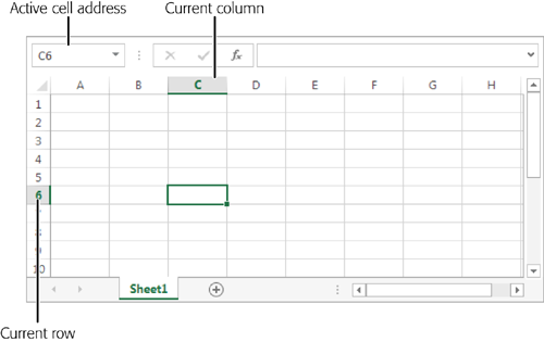
Figure 1-3. In this spreadsheet, the active cell is C6. You can recognize an active (or current) cell by its heavy black border. Youâll also notice that Excel highlights the corresponding column letter (C) and row number (6) at the edges of the worksheet. Just above the worksheet, on the left side of the window, the formula bar gives you the active cellâs address.
The best way to get a feel for Excel is to dive right in and start putting together a worksheet. The following sections cover each step that goes into assembling a simple worksheet. This one tracks household expenses, but you can use the same approach with any basic worksheet.
Excel lets you arrange information in whatever way you like. Thereâs nothing to stop you from scattering numbers left and right, across as many cells as you want. However, one of the most common (and most useful) ways to arrange information is in a table, with headings for each column.
Itâs important to remember that with even the simplest worksheet, the decisions you make about whatâs going to go in each column can have a big effect on how easy it is to manipulate your information. For example, in a worksheet that stores a mailing list, you could have two columns: one for names and another for addresses. But if you create more than two columns, your life will probably be easier because you can separate first names from street addresses from ZIP codes, and so on. Figure 1-4 shows the difference.
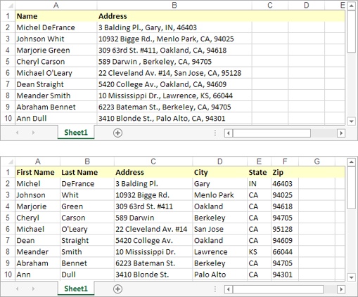
Figure 1-4. Top: If you enter both first and last names in a single column, you can sort the column only by first name. And if you clump the addresses and ZIP codes together, you have no way to count the number of people in a certain town or neighborhood. Bottom: The benefit of a six-column table is significant: It lets you break down (and therefore analyze) information granularly, For example, you can sort your list according to peopleâs last names or where they live. This arrangement also lets you filter out individual bits of information when you start using functions later in this book.
You can, of course, always add or remove columns. But you can avoid getting gray hairs by starting a worksheet with all the columns you think youâll need.
The first step in creating a worksheet is to add your headings in the row of cells at the top of the sheet (row 1). Technically, you donât need to start right in the first row, but unless you want to add more information before your tableâlike a title for the chart or todayâs dateâthereâs no point in wasting space. Adding information is easyâjust click the cell you want and start typing. When you finish, hit Tab to complete your entry and move to the cell to the right, or click Enter to head to the cell just underneath.
Note
The information you put in an Excel worksheet doesnât need to be in neat, ordered columns. Nothing stops you from scattering numbers and text in random cells. However, most Excel worksheets resemble some sort of table, because thatâs the easiest and most effective way to manage large amounts of structured information.
For a simple expense worksheet designed to keep a record of your most prudent and extravagant purchases, try the following three headings:
Right away, you face your first glitch: awkwardly crowded text. Figure 1-5 shows how to adjust the column width for proper breathing room.
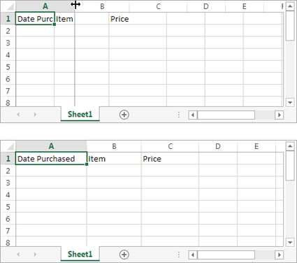
Figure 1-5. Top: The standard width of an Excel column is 8.43 characters, which hardly allows you to get a word in edgewise. Hereâs how to give yourself some more room. First, position your mouse on the right border of the column header you want to expand so that the mouse pointer changes to the resize icon (it looks like a double-headed arrow). Now drag the column border to the right as far as you want. As you drag, a tooltip appears, telling you the character size and pixel width of the column. Both of these pieces of information play the same roleâthey tell you how wide the column is. Only the unit of measurement changes. Bottom: When you release the mouse, Excel resizes the entire column of cells to the new width.
Note
A columnâs character width doesnât really reflect how many characters (or letters) fit in a cell. Excel uses proportional fonts, in which different letters take up different amounts of room. For example, the letter W is typically much wider than the letter I. All this means is that the character width Excel shows you isnât a real indication of how many letters can fit in the column, but itâs a useful way to compare column widths.
You can now begin adding your data: Simply fill in the rows under the column titles. Each row in the expense worksheet represents a separate purchase. (If youâre familiar with databases, you can think of each row as a separate record.)
As Figure 1-6 shows, the first column is for dates, the second stores text, and the third holds numbers. Keep in mind that Excel doesnât impose any rules on what you type, so youâre free to put text in the Price column. But if you donât keep a consistent kind of data in each column, you wonât be able to easily analyze (or understand) your information later.
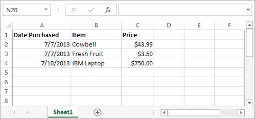
Figure 1-6. This rudimentary expense list has three items in it (in rows 2, 3, and 4). By default, Excel aligns the items in a column according to their data type. It aligns numbers and dates on the right, and text on the left.
Thatâs it. Youâve now created a living, breathing worksheet. The next section explains how you can edit the data you just entered.
Every time you start typing in a cell, Excel erases any existing content in that cell. (You can also quickly remove the contents of a cell by moving to the cell and pressing Delete, which clears its contents.)
If you want to edit cell data instead of replacing it, you need to put the cell in edit mode, like this:
Move to the cell you want to edit.
Use the mouse or the arrow keys to get to the correct cell.
Put the cell in edit mode by pressing F2 or by double-clicking inside it.
Edit mode looks like ordinary text-entry mode, but you can use the arrow keys to position your cursor in the text youâre editing. (When you arenât in edit mode, pressing these keys just moves you to another cell.)
Complete your edit.
Once you modify the cell content, press Enter to confirm your changes or Esc to cancel your edit and leave the old value in the cell. Alternatively, you can click on another cell to accept the current value and go somewhere else. But while youâre in edit mode, you canât use the arrow keys to move out of the cell.
Tip
If you start typing new information into a cell and you decide you want to move to an earlier position in your entry (to make an alteration, for instance), just press F2. The cell box still looks the same, but now youâre in edit mode, which means that you can use the arrow keys to move within the cell (instead of going from cell to cell). Press F2 again to return to data entry mode, where you can use the arrow keys to move to other cells.
As you enter data, you may discover the Bigtime Excel Display Problem (known to aficionados as BEDP): Cells in adjacent columns can overlap one another. Figure 1-7 illustrates the problem. One way to fix BEDP is to manually resize the column, as shown in Figure 1-5. Another option is to turn on text wrapping so you can fit multiple lines of text in a single cell, as described on Alignment and Orientation.
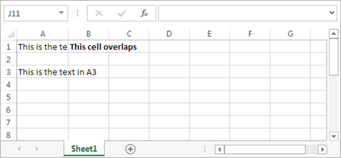
Figure 1-7. Overlapping cells can create big headaches. For example, if you type a large amount of text into A1 and then you type some text into B1, you see only part of A1âs data in your worksheet (as shown here). The rest is hidden from view. But if, say, A3 contains a large amount of text and B3 is empty, Excel displays the content in A3 over both columns, and you donât have a problem.
Just above the worksheet grid but under the ribbon is an indispensable editing tool called the formula bar (Figure 1-8). It displays the address of the active cell (like A1) on the left edge, and it shows you the current cellâs contents.
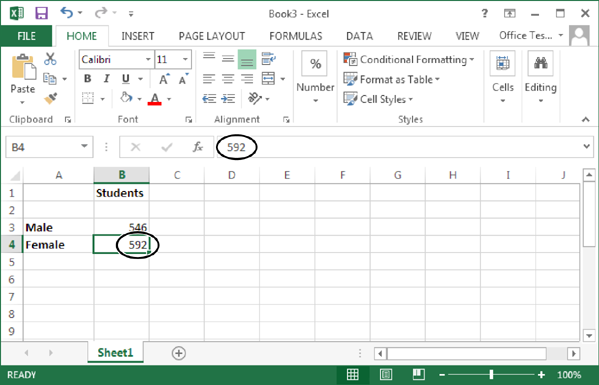
Figure 1-8. The formula bar (just above the grid) displays information about the active cell. In this example, you can see that the current cell is B4 and it contains the number 592. Instead of editing this value in the cell, you can click anywhere in the formula bar and make your changes there.
You can use the formula bar to enter and edit data instead of editing directly in your worksheet. This is particularly useful when a cell contains a formula or a large amount of information. Thatâs because the formula bar gives you more work room than a typical cell. Just as with in-cell edits, you press Enter to confirm formula bar edits or Esc to cancel them. Or you can use the mouse: When you start typing in the formula bar, a checkmark and an âXâ icon appear just to the left of the box where youâre typing. Click the checkmark to confirm your entry or âXâ to roll it back.
Ordinarily, the formula bar is a single line. If you have a really long entry in a cell (like a paragraphâs worth of text), you need to scroll from one side to the other. However, thereâs another optionâyou can resize the formula bar so that it fits more information, as shown in Figure 1-9.
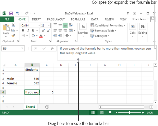
Figure 1-9. To enlarge the formula bar, click the bottom edge and pull down. You can make it two, three, four, or many more lines large. Best of all, once you get the size you want, you can use the expand/collapse button to the right of the formula bar to quickly expand it to your preferred size and collapse it back to the single-line view.
The focal point of the Excel window is the worksheet grid. Itâs where you enter and edit information, whether thatâs an amortization table for a business loan or a catalog of your rare Spider-Man comics. However, it wonât be long before you need to direct your attention upwards, to the super-toolbar that sits at the top of the Excel window. This is the ribbon, and it ensures that even the geekiest Excel features are only a click or two away.
Everything youâll ever want to do in Excelâfrom picking a fancy background color to pulling information out of a databaseâis packed into the ribbon. To accommodate all these buttons without becoming an over-stuffed turkey, the ribbon uses tabs. You start out with seven tabs. When you click one, you see a whole new collection of buttons (Figure 1-10).
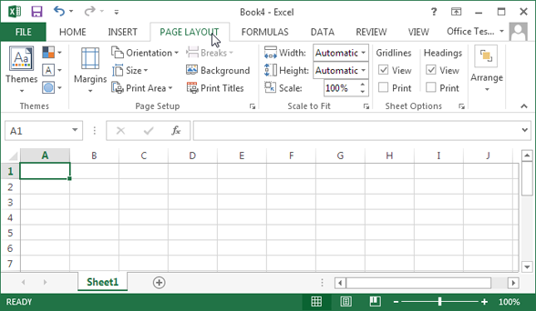
Figure 1-10. When you launch Excel, you start at the Home tab. But hereâs what happens when you click the Page Layout tab. Now, you have a slew of options for tasks like adjusting paper size and making a decent printout. Excel groups the buttons within a tab into smaller sections for clearer organization.
The ribbon makes it easy to find features because Excel groups related features under the same tab. Even better, once you find the button you need, you can often find other, associated commands by looking at the other buttons in the tab. In other words, the ribbon isnât just a convenient tool, itâs also a great way to explore Excel.
The ribbon is full of craftsman-like detail. For example, when you hover over a button, you donât see a paltry two- or three-word description in a yellow rectangle. Instead, you see a friendly pop-up box with a mini-description of the feature and (often) a shortcut that lets you trigger the command from the keyboard. Another nice detail is the way you can jump from one tab to another at high velocity by positioning your mouse pointer over the ribbon and rolling the scroll wheel (if your mouse has a scroll wheel). And youâre sure to notice the way the ribbon rearranges its buttons when you change the size of the Excel window (see Figure 1-11).
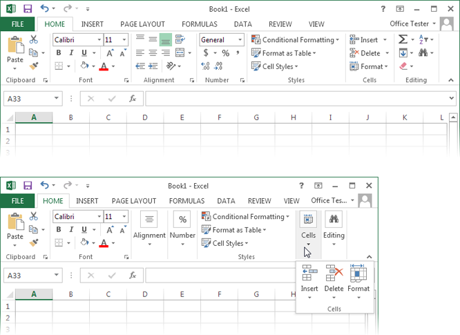
Figure 1-11. Top: A large Excel window gives you plenty of room to play. The ribbon uses the space effectively, making the most important buttons bigger. Bottom: When you shrink the Excel window, the ribbon shrinks some buttons or hides their text to make room. Shrink small enough, and Excel starts to replace cramped sections with a single button, like the Alignment, Cells, and Editing sections shown here. Click the button and the missing commands appear in a drop-down panel.
Throughout this book, youâll dig through the ribbonâs tabs to find important features. But before you start your journey, hereâs a quick overview of what each tab provides.
File isnât really a toolbar tab, even though it appears first in the list. Instead, itâs your gateway to Excelâs backstage view, as described on Going Backstage.
Home includes some of the most commonly used buttons, like those for cutting and pasting text, formatting data, and hunting down important information with search tools.
Insert lets you add special ingredients to your spreadsheets, like tables, graphics, charts, and hyperlinks.
Page Layout is all about getting your worksheet ready for printing. You can tweak margins, paper orientation, and other page settings.
Formulas are mathematical instructions that perform calculations. This tab helps you build super-smart formulas and resolve mind-bending errors.
Data lets you get information from an outside data source (like a heavy-duty database) so you can analyze it in Excel. It also includes tools for dealing with large amounts of information, like sorting, filtering, and subgrouping data.
Review includes the familiar Office proofing tools (like the spell-checker). It also has buttons that let you add comments to a worksheet and manage revisions.
View lets you switch on and off a variety of viewing options. It also lets you pull off a few fancy tricks if you want to view several separate Excel spreadsheet files at the same time; see Viewing Multiple Workbooks at Once.
Note
In some circumstances, you may see tabs that arenât in this list. Macro programmers and other highly technical types use the Developer tab. (Youâll learn how to reveal this tab on Attaching a Macro to a Button Inside a Worksheet.) The Add-Ins tab appears when you open workbooks created in previous versions of Excel that use custom toolbars. And finally, you can create a tab of your own if youâre ambitious enough to customize the ribbon, as explained in the Appendix.
Most people are happy to have the ribbon sit at the top of the Excel window, with all its buttons on hand. But serious number-crunchers demand maximum space for their dataâtheyâd rather look at another row of numbers than a pumped-up toolbar. If this describes you, then youâll be happy to find out that you can collapse the ribbon, which shrinks it down to a single row of tab titles, as shown in Figure 1-12. To collapse it, just double-click the current tab title. (Or click the tiny up-pointing icon in the top-right corner of the ribbon, right next to the help icon.)
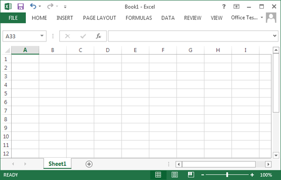
Figure 1-12. Do you want to use every square inch of screen space for your cells? You can collapse the ribbon (as shown here) by double-clicking any tab. Click a tab to pop it open temporarily, or double-click a tab to bring the ribbon back for good. And if you want to perform the same trick without lifting your fingers from the keyboard, use the shortcut Ctrl+F1.
Even if you collapse the ribbon, you can still use all its features. All you need to do is click a tab. For example, if you click Home, the Home tab pops open over your worksheet. As soon as you click the button you want in the Home tab (or click a cell in your worksheet), the ribbon collapses again. The same trick works if you trigger a command in the ribbon using the keyboard, as described in the next section.
If you use the ribbon only occasionally, or if you prefer to use keyboard shortcuts, it makes sense to collapse the ribbon. Even then, you can still use the ribbon commandsâit just takes an extra click to open the tab. On the other hand, if you make frequent trips to the ribbon or youâre learning about Excel and like to browse the ribbon to see what features are available, donât bother collapsing it. The two or three spreadsheet rows youâll lose are well worth it.
If youâre an unredeemed keyboard lover, youâll be happy to hear that you can trigger ribbon commands with the keyboard. The trick is using keyboard accelerators, a series of keystrokes that starts with the Alt key (the same key you used to use to get to a menu). When you use a keyboard accelerator, you donât hold down all the keys at the same time. (As youâll soon see, some of these keystrokes contain so many letters that youâd be playing Finger Twister if you tried.) Instead, you hit the keys one after the other.
The trick to keyboard accelerators is understanding that once you hit the Alt key, there are two things you do, in this order:
Pick the ribbon tab you want.
Choose a command in that tab.
Before you can trigger a specific command, you must select the correct tab (even if itâs already selected). Every accelerator requires at least two key presses after you hit the Alt key. You need to press even more keys to dig through submenus.
By now, this whole process probably seems hopelessly impractical. Are you really expected to memorize dozens of accelerator key combinations?
Fortunately, Excel is ready to help you out with a feature called KeyTips. Hereâs how it works: When you press Alt, letters magically appear over every tab in the ribbon. Once you hit the corresponding key to pick a tab, letters appear over every button in that tab (Figure 1-13). Once again, you press the corresponding key to trigger the command (Figure 1-14).
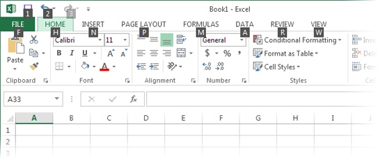
Figure 1-13. When you press Alt, Excel displays KeyTips next to every tab, over the File menu, and over the buttons in the Quick Access toolbar. If you follow up with M (for the Formulas tab), youâll see letters next to every command in that tab, as shown in Figure 1-11.
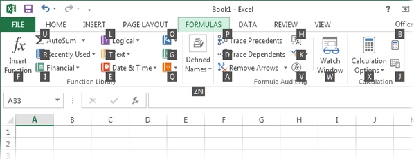
Figure 1-14. You can now follow up with F to trigger the Insert Function button, U to get to the AutoSum feature, and so on. Donât bother trying to match letters with tab or button namesâthere are so many features packed into the ribbon that in many cases the letters donât mean anything at all.
Sometimes, a command might have two letters, in which case you need to press both keys, one after the other. (For example, the Find & Select button on the Home tab has the letters FD. To trigger it, press Alt, then H, then F, and then D.)
Tip
You can go back one step in KeyTips mode by pressing Esc. Or, you can stop cold without triggering a command by pressing Alt again.
Excel gives you other shortcut keys that donât use the ribbon. These are key combinations that start with the Ctrl key. For example, Ctrl+C copies highlighted text, and Ctrl+S saves your work. Usually, you find out about a shortcut key by hovering over a command with your mouse. For example, hover over the Paste button in the ribbonâs Home tab, and you see a tooltip that tells you its timesaving shortcut key, Ctrl+V. And if you worked with a previous version of Excel, youâll find that Excel 2013 uses almost all the same shortcut keys.
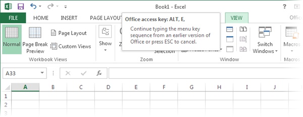
Figure 1-15. When you press Alt+E in Excel 2013, you trigger the âimaginaryâ Edit menu originally in Excel 2003 and earlier. You canât actually see the menu, because it doesnât exist in Excel 2013, but the tooltip lets you know that Excel is paying attention. You can now complete your action by pressing the next key for the menu command youâre nostalgic for.
Keen eyes will have noticed the tiny bit of screen real estate just above the ribbon. It holds a series of tiny icons, like the toolbars in older versions of Excel (Figure 1-16). This is the Quick Access toolbar (or QAT, to Excel nerds).
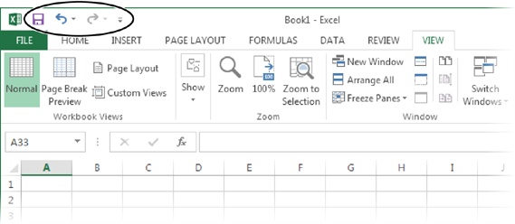
Figure 1-16. The Quick Access toolbar puts the Save, Undo, and Redo commands right at your fingertips. Excel provides easy access to these commands because most people use them more frequently than any others. But as youâll learn in the Appendix, you can add any commands you want here.
If the Quick Access toolbar were nothing but a specialized shortcut for three commands, it wouldnât be worth the bother. But it has one other notable attribute: You can customize it. In other words, you can remove commands you donât use and add your own favorites. The Appendix of this book (Creating Custom Functions) shows you how.
Microsoft has deliberately kept the Quick Access toolbar very small. Itâs designed to provide a carefully controlled outlet for those customization urges. Even if you go wild stocking the Quick Access toolbar with your own commands, the rest of the ribbon remains unchanged. (And that means a co-worker or spouse can still use Excel, no matter how dramatically you change the QAT.)
Though people often overlook it, Excelâs status bar (Figure 1-17) is a good way to monitor the programâs current state. For example, if you save or print a document, the status bar shows the progress of the save operation or print job. If your task is simple, the progress indicator may disappear before you even have a chance to notice it. But if youâre performing a time-consuming operationâsay, printing an 87-page table of the hotel silverware you happen to ownâyou can look to the status bar to see how things are coming along.
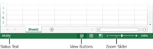
Figure 1-17. In the status bar, you can see the basic status text (which just says âReadyâ in this example), the view buttons (useful as you prepare a spreadsheet for printing), and the zoom slider (which lets you enlarge or shrink the current worksheet).
The status bar combines several types of information. The leftmost area shows Cell Mode, which displays one of three indicators:
Ready means that Excel isnât doing anything much at the moment, other than waiting to execute a command.
Enter appears when you start typing a new value into a cell.
Edit means you currently have the cell in edit mode, and pressing the left and right arrow keys moves through the data within a cell, instead of moving from cell to cell. You can place a cell in edit mode or take it out of edit mode by pressing F2.
Farther to the right of the status bar are the view buttons, which let you switch to Page Layout view or Page Break Preview. These help you see what your worksheet will look like when you print it. Theyâre covered in Chapter 7.
The zoom slider is next to the view buttons, at the far right edge of the status bar. You can slide it to the left to zoom out (which fits more information into your Excel window) or slide it to the right to zoom in (and take a closer look at fewer cells). You can learn more about zooming on Zooming.
In addition, the status bar displays other miscellaneous indicators. If you press the Scroll Lock key, for example, a Scroll Lock indicator appears in the status bar (next to the âReadyâ text). This indicator tells you that youâre in scroll mode, where the arrow keys donât move you from one cell to another, but scroll the entire worksheet up, down, or to the side. Scroll mode is a great way to check out another part of your spreadsheet without leaving your current position.
You can control what indicators appear in the status bar by configuring it. To see the list of possibilities, right-click the status bar (Figure 1-8). Table 1-2 describes the options.
Table 1-1. Status bar indicators
MEANING | |
|---|---|
Shows Ready, Edit, or Enter depending on the state of the current cell. | |
Shows the number of cells that were skipped (left blank) and the number of cells that were filled after a Flash Fill operation (Flash Fill). | |
Displays information about the rights and restrictions of the current spreadsheet. These features come into play only if you use a SharePoint server to share spreadsheets among groups of people (usually in a corporate environment). | |
Caps Lock | Indicates whether you have Caps Lock mode on. When it is, Excel automatically capitalizes every letter you type. To turn Caps Lock on or off, hit the Caps Lock key. |
Num Lock | Indicates whether Num Lock mode is on. When it is, you can use the numeric keypad (typically on the right side of your keyboard) to type in numbers more quickly. When this signâs off, the numeric keypad controls cell navigation instead. To turn Num Lock on or off, press Num Lock. |
Scroll Lock | Indicates whether Scroll Lock mode is on. When itâs on, you can use the arrow keys to scroll through a worksheet without changing the active cell. (In other words, you can control your scrollbars by just using your keyboard.) This feature lets you look at all the information in your worksheet without losing track of the cell youâre currently in. You can turn Scroll Lock mode on or off by pressing Scroll Lock. |
Fixed Decimal | Indicates when Fixed Decimal mode is on. When it is, Excel automatically adds a set number of decimal places to the values you enter in any cell. For example, if you tell Excel to use two fixed decimal places and you type the number 5 into a cell, Excel actually enters 0.05. This seldom-used featured is handy for speed typists who need to enter reams of data in a fixed format. You can turn this feature on or off by selecting FileâOptions, choosing the Advanced section, and then looking under âEditing optionsâ to find the âAutomatically insert a decimal pointâ setting. Once you turn this checkbox on, you can choose the number of decimal places displayed (the standard option is 2). |
Indicates when you have Overwrite mode turned on. Overwrite mode changes how cell edits work. When you edit a cell with Overwrite mode on, the new characters that you type overwrite existing characters (rather than displacing them). You can turn Overwrite mode on or off by pressing Insert. | |
Indicates that youâve pressed End, which is the first key in many two-key combinations; the next key determines what happens. For example, hit End and then Home to move to the bottom-right cell in your worksheet. | |
Macros are automated routines that perform some task in an Excel spreadsheet. The Macro Recording indicator shows a record button (which looks like a red circle superimposed on a worksheet) that lets you start recording a new macro. Youâll learn more about macros in Chapter 29. | |
Indicates the current Selection mode. You have two options: normal mode and extended selection. When you press the arrows keys with Extended selection on, Excel automatically selects all the rows and columns you cross as you move around the spreadsheet. Extended selection is a useful keyboard alternative to dragging your mouse to select swaths of the grid. To turn Extended selection on or off, press F8. Youâll learn more about selecting cells and moving them around in Chapter 3. | |
Shows the current page and the total number of pages (as in âSafari© Books Online of 4â). This indicator appears only in Page Layout view (as described on Page Layout View: A Better Print Preview). | |
Show the result of a calculation on selected cells. For example, the Sum indicator totals the value of all the numeric cells selected. Youâll take a closer look at this handy trick on Making Continuous Range Selections. | |
Does nothing (that we know of). Excel does show a handy indicator in the status bar when youâre uploading files to the Web, as youâll learn in Chapter 26. However, Excel always displays the upload status when needed, and this setting doesnât seem to have any effect. | |
View Shortcuts | Shows the three view buttons that let you switch between Normal view, Page Layout view, and Page Break Preview. |
Zoom | Shows the current zoom percentage (like 100 percent for a normal-sized spreadsheet, and 200 percent for a spreadsheet thatâs blown up to twice the magnification). |
Lets you zoom in (by moving the slider to the right) or out (by moving it to the left) to see more information at once. |
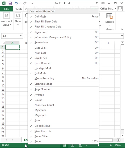
Figure 1-18. Every item that has a checkmark appears in the status bar when you need it. For example, if you choose Caps Lock, the text âCaps Lockâ appears in the status bar whenever you hit the Caps Lock key. The text that appears on the right side of the list tells you the current value of the indicator. In this example, Caps Lock mode is currently off and the Cell Mode text says âReady.â
Your data is the star of the show. Thatâs why the creators of Excel refer to your worksheet as being âon stage.â The auditorium is the Excel main window, whichâas youâve just seenâincludes the handy ribbon, formula bar, and status bar. Sure, itâs a strange metaphor. But once you understand it, youâll realize the rationale for Excelâs backstage view, which temporarily takes you away from your worksheet and lets you concentrate on other tasks that donât involve entering or editing data. These tasks include saving your spreadsheet, opening more spreadsheets, printing your work, and changing Excelâs settings.
To switch to backstage view, click the File button to the left of the Home ribbon tab. Excel temporarily tucks your worksheet out of sight (although itâs still open and waiting for you). This gives Excel the space it needs to display information related to the task at hand, as shown in Figure 1-19. For example, if you plan to print your spreadsheet, Excelâs backstage view previews the printout. Or if you want to open an existing spreadsheet, Excel can display a detailed list of files you recently worked on.
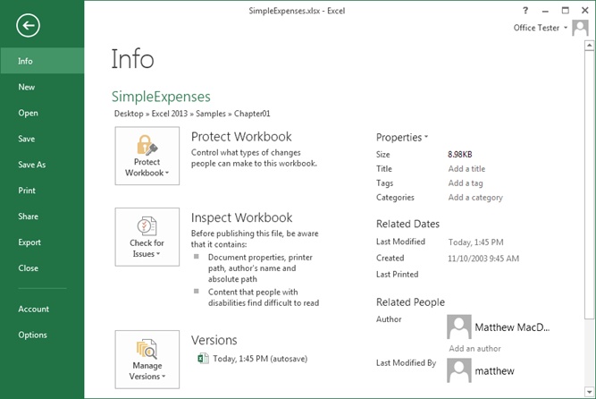
Figure 1-19. When you first switch to backstage view, Excel shows the Info page, which provides basic information about your workbook file, its size, when it was last edited, who edited it, and so on (see the column on the far right). The Info page also provides the gateway to three important features: document protection (Chapter 21), compatibility checking (page 31), and AutoRecover backups (page 38). To go to another section, click a different command in the column on the far left.
To get out of backstage view and return to your worksheet, press Esc or click the arrow-in-a-circle icon in the top-right corner of backstage view.
The key to using backstage view is the menu of commands that runs in a strip along the left side of the window. You click a command to get to the page for the task you want to perform. For example, to create a new spreadsheet (in addition to the one youâre currently working on), you begin by clicking the New command, as shown in Figure 1-20.
Tip
You donât need to go to backstage view to create a new, blank spreadsheet. Instead, hit the shortcut key Ctrl+N while youâre in the worksheet grid. Excel will launch a new window, with a new, blank worksheet at the ready.
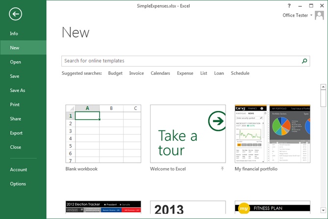
Figure 1-20. When you click New, you see a page resembling the welcome page that greets you when you start Excel. To create a new, empty workbook, click âBlank workbook.â Excel opens the workbook in a new window, so that itâs separate from your current workbook, which Excel leaves untouched.
Here are some of the things youâll do in Excelâs backstage view:
Work with files (create, open, close, and save them) with the help of the New, Open, Save, and Save As commands. Youâll spend the rest of this chapter learning the fastest and most effective ways to save and open Excel files.
Print your work (Chapter 7) and email it to other people (Chapter 25) using the Print and Share commands.
Prepare a workbook you want to share with others. For example, you can check its compatibility with older versions of Excel (Chapter 1) and lock your document to prevent other people from changing numbers (Chapter 24). You find these options under the Info command.
Configure your Office accountâthatâs the email address and password you use to access Microsoftâs SkyDrive service for storing spreadsheets online (Introducing SkyDrive) or for your Office 365 account (if youâre a subscriber; see page xvii). To do this, click the Account command.
Configure how Excel behaves. Once youâre in backstage view, click Options to launch the Excel Options window, an all-in-one place for configuring Excel.
As everyone whoâs been alive for at least three days knows, you should save your work early and often. Excel is no exception. To save a file for the first time, choose FileâSave or FileâSave As. Either way, you end up at the Save As page in backstage view (Figure 1-21).
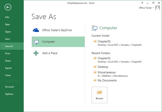
Figure 1-21. The first time you save your spreadsheet, you need to choose where to put it. Usually, youâll pick a location on your hard drive (click Computer in the Places list), but you can upload it to a corporate SharePoint service or to Microsoftâs SkyDrive for online sharing almost as easily.
The Save As window includes a list of placesâlocations where you can store your work. The exact list depends on how you configured Excel, but here are some of the options youâre likely to see:
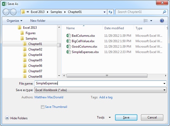
Computer. Choose this to store your spreadsheet somewhere on your computerâs hard drive. This is the most common option. When you click Computer, Excel lists the folders where you recently saved or opened files (see Figure 1-21, on the right). To save a file to one of these locations, select the folder. Or, click the big Browse button at the bottom to find a new location. Either way, Excel opens the familiar Save As window, where you type in a name for your file (Figure 1-22).
SkyDrive. When you set up Excel, you can supply the email address and password you use for Microsoft services like Hotmail, Messenger, and SkyDrive, Microsoftâs online file-storage system. Excel features some nifty SkyDrive integration features. For example, you can upload a spreadsheet straight to the Web by clicking your personalized SkyDrive item in the Places list, and then choosing one of your SkyDrive folders.
Note
The advantage of putting a file on SkyDrive is that you can open and edit it from another Excel-equipped computer, without needing to worry about copying or emailing the file. The other advantage is that other people can edit your file with the Excel Web App. Youâll learn more about SkyDrive and the Excel Web App in Chapter 23.
SharePoint. If youâre running a computer on a company network, you may be able to store your work on a SharePoint server. Doing so not only lets you share your work with everyone else on your team, it lets you tap into SharePointâs excellent workflow features. (For example, your organization could have a process set up where you save expense reports to a SharePoint server, and theyâre automatically passed on to your boss for approval and then accounting for payment.) A SharePoint server wonât necessarily have the word âSharePointâ in its place name, but it will have the globe-and-server icon to let you know itâs a web location.
After you save a spreadsheet once, you can quickly save it again by choosing FileâSave, or by pressing Ctrl+S. Or look up at the top of the Excel window in the Quick Access toolbar for the tiny Save button, which looks like an old-style diskette. To save your spreadsheet with a new name or in a new place, select FileâSave As, or press F12.
Tip
Saving a spreadsheet is an almost instantaneous operation, and you should get used to doing it regularly. After you make any significant change to a sheet, hit Ctrl+S to store the latest version of your data.
Ordinarily, youâll save your spreadsheets in the modern .xlsx format, which is described in the next section. However, sometimes youâll need to convert your spreadsheet to a different type of fileâfor example, if you want to pass them along to someone using a very old version of Excel, or a different type of spreadsheet program. There are two ways you can do this:
Choose FileâSave As and pick a location. Then, in the Save As window (Figure 1-22), click âSave as typeâ and then pick the format you want from the long drop-down list.
Choose FileâExport, and then click Change File Type. Youâll see a list of the 10 most popular formats. Click one to open a Save As window with that format selected. Or, if you donât see the format you want, click the big Save As button underneath to open a Save As window, and then pick the format yourself from the âSave as typeâ drop-down list.
Excel lets you save your spreadsheet in a variety of formats, including the classic Excel 95 format from more than a decade ago. If you want to look at your spreadsheet using a mystery program, use the CSV file type, which produces a comma-delimited text file that almost all spreadsheet programs can read (comma-delimited means that commas separate the information in each cell). And in the following sections, youâll learn more about sharing your work with old versions of Excel (Sharing Your Spreadsheet with Older Versions of Excel) or putting it in PDF form so anyone can view and print it (Saving Your Spreadsheet As a PDF). But first, you need to take a closer look at Excelâs standard file format.
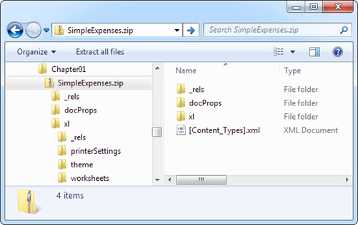
Modern versions of Excel, including Excel 2013, use the .xlsx file format (which means your saved spreadsheet will have a name like HotelSilverware.xlsx). Microsoft introduced this format in Excel 2007, and it comes with significant advantages:
Itâs compact. The .xlsx format uses ZIP file compression, so spreadsheet files are smallerâas much as 75 percent smaller than Excel 2003 files. And even though the average hard drive is already large enough to swallow millions of old-fashioned Excel files, a more compact format is easier to share online and via email.
Itâs less error-prone. The .xlsx format carefully separates ordinary content, pictures, and macro code into separate sections. That means that if a part of your Excel file is damaged (due to a faulty hard drive, for example), thereâs a good chance that you can still retrieve the rest of the information. (Youâll learn about Excel disaster recovery on Disaster Recovery.)
Itâs extensible. The .xlsx format uses XML (the eXtensible Markup Language), which is a standardized way to store information. (Youâll learn more about XML in Chapter 28.) XML storage doesnât benefit the average person, but itâs sure to earn a lot of love from companies that use custom software in addition to Excel. As long as you store the Excel documents in XML format, these companies can create automated programs that pull the information they need straight out of the spreadsheet, without going through Excel itself. These programs can also generate made-to-measure Excel documents on their own.
For all these reasons, .xlsx is the format of choice for Excel 2013. However, Microsoft prefers to give people all the choices they could ever need (rather than make life really simple), and Excel file formats are no exception. In fact, the .xlsx file format actually comes in two additional flavors.
First, thereâs the closely related .xlsm, which lets you store macro code with your spreadsheet data. If you add macros to a spreadsheet, Excel prompts you to use this file type when you save your work. (Youâll learn about macros in Chapter 29.)
Second, thereâs the optimized .xlsb format, which is a specialized option that might be a bit faster when opening and saving gargantuan spreadsheets. The .xlsb format has the same automatic compression and error-resistance as .xlsx, but it doesnât use XML. Instead, it stores information in raw binary form (good olâ ones and zeros), which is speedier in some situations. To use the .xlsb format, choose FileâExport, click Change File Type, and then choose âBinary Workbook (.xlsb)â from the drop-down list.
Most of the time, you donât need to think about Excelâs file format. You can just create your spreadsheets, save them, and let Excel take care of the rest. The only time you need to stop and think twice is when you share your work with other, less fortunate people who have older versions of Excel, such as Excel 2003. Youâll learn how to deal with this challenge in the following sections.
Tip
Donât use the .xlsb format unless you try it out and find that it really does give you better performance. Usually, .xlsx and .xlsb are just as fast. And remember, the only time youâll see any improvement is when you load or save a file. Once you open your spreadsheet in Excel, everything else (like scrolling around and performing calculations) happens at the same speed.
As you just learned, Excel 2013 uses the same .xlsx file format as Excel 2010 and Excel 2007. That means that an Excel 2013 fan can exchange files with an Excel 2010 devotee, and there wonât be any technical problems.
However, a few issues can still trip you up when you share spreadsheets between different versions of Excel. For example, Excel 2013 introduces a few new formula functions, such as BASE (BASE() and DECIMAL(): Converting Numbers to Different Bases). If you write a calculation in Excel 2013 that uses BASE(), the calculation wonât work in Excel 2010. Instead of seeing the numeric result you want, your recipient will see an error code mixed in with the rest of the spreadsheet data.
To avoid this sort of problem, you need the help of an Excel tool called the Compatibility Checker. It scans your spreadsheet for features and formulas that will cause problems in Excel 2010 or Excel 2007.
To use the Compatibility Checker, follow these steps:
Choose FileâInfo.
Excel switches into backstage view.
Click the Check for Issues button, and choose Check Compatibility.
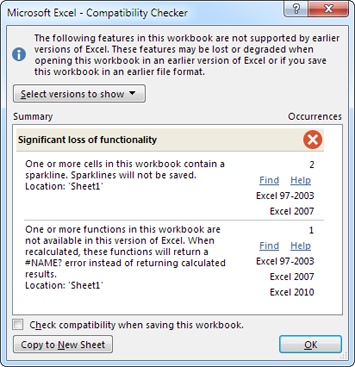
The Compatibility Checker scans your spreadsheet, looking for signs of trouble. It reports problems to you (Figure 1-24).
Optionally, you can choose to hide compatibility problems that donât affect you.
The Compatibility Checker reports on three types of problems:
You donât necessarily need to worry about all these versions of Excel. For example, if you plan to share your files with Excel 2010 users but not with people using Excel 2007 or older, you donât need to pay attention to the first two categories, because they donât affect your peeps.
To choose what errors the Compatibility Checker reports on, click the âSelect versions to showâ button and turn off the checkboxes next to the versions of Excel you donât want to consider. For example, you can turn off âExcel 97-2003â if you donât want to catch problems that affect only these versions of Excel.
Review the problems.
You can ignore the Compatibility Checker issues, click Find to hunt each one down, or click Help to figure out the exact problem. You can also click âCopy to New Sheetâ to insert a full compatibility report into your spreadsheet as a separate worksheet. This way, you can print it up and review it in the comfort of your cubicle. (To get back to the worksheet with your data, click the Sheet1 tab at the bottom of the window. Chapter 4 has more about how to use and manage multiple worksheets.)
Note
The problems that the Compatibility Checker finds wonât cause serious errors, like crashing your computer or corrupting your data. Thatâs because Excel is designed to degrade gracefully. That means you can still open a spreadsheet that uses newer, unsupported features in an old version of Excel. However, you may receive a warning message and part of the spreadsheet may seem brokenâthat is, it wonât work as you intended.
Optionally, you can set the Compatibility Checker to run automatically for this workbook.
Turn on the âCheck compatibility when saving this workbookâ checkbox. Now, the Compatibility Checker runs each time you save your spreadsheet, just before Excel updates the file.
Once your work passes through the Compatibility Checker, youâre ready to save it. Because Excel 2013, Excel 2010, and Excel 2007 all share the same file format, you donât need to perform any sort of conversionâjust save your file normally. But if you want to share your spreadsheet with Excel 2003, follow the instructions in the next section.
Sharing your workbook with someone using Excel 2003 presents an additional consideration: Excel 2003 uses the older .xls format instead of the current-day .xlsx format.
There are two ways to resolve this problem:
Save your spreadsheet in the old format. You can save a copy of your spreadsheet in the traditional .xls standard Microsoft has supported since Excel 97. To do so, choose FileâExport, click Change File Type, and choose âExcel 97-2003 Workbook (*.xls)â from the list of file types.
Use a free add-in for older versions of Excel. People stuck with Excel 2000, Excel 2002, or Excel 2003 can read your Excel 2013 filesâthey just need a free add-in from Microsoft. This is a good solution because it doesnât require you to do extra work, like saving both a current and a backward-compatible version of the spreadsheet. People with past-its-prime versions of Excel can find the add-in by surfing to www.microsoft.com/downloads and searching for âcompatibility pack file formatsâ (or use the secret shortcut URL tinyurl.com/y5w78r). However, you should still run the Compatibility Checker to find out if your spreadsheet uses features that Excel 2003 doesnât support.
Tip
If you save your Excel spreadsheet in the Excel 2003 format, make sure to keep a copy in the standard .xlsx format. Why? Because the old format isnât guaranteed to retain all your information, particularly if you use newer chart features or data visualization.
As you already know, each version of Excel introduces a small set of new features. Older versions donât support these features. The differences between Excel 2010 and Excel 2013 are small, but the differences between Excel 2003 and Excel 2013 are more significant.
Excel tries to help you out in two ways. First, whenever you save a file in .xls format, Excel automatically runs the Compatibility Checker to check for problems. Second, whenever you open a spreadsheet in the old .xls file format, Excel switches into compatibility mode. While the Compatibility Checker points out potential problems after the fact, compatibility mode is designed to prevent you from using unsupported features in the first place. For example, in compatibility mode youâll face these restrictions:
Excel limits you to a smaller grid of cells (65,536 rows instead of 1,048,576).
Excel prevents you from using really long or deeply nested formulas.
Excel doesnât let you use some pivot table features.
In compatibility mode, these missing features arenât anywhere to be found. In fact, compatibility mode is so seamless that you might not even notice its limitations. The only clear indication that youâre in Compatibility Mode appears at the title bar at the top of the Excel window. Instead of seeing something like CateringList.xlsx, youâll see âCateringList.xls [Compatibility Mode].â
Note
When you save an Excel workbook in .xls format, Excel wonât switch into compatibility mode right away. Instead, you need to close the workbook and reopen it.
If you decide at some point that youâre ready to move into the modern world and convert your file to the .xlsx format favored by Excel 2013, you can use the trusty FileâSave As command. However, thereâs an even quicker shortcut. Just choose FileâInfo and click the Convert button. This saves an Excel 2013 version of your file with the same name but with the extension .xlsx, and reloads the file so you get out of compatibility mode. Itâs up to you to delete your old .xls original if you donât need it anymore.
Sometimes you want to save a copy of your spreadsheet so that people can read it even if they donât have Excel (and even if theyâre running a different operating system, like Linux or Appleâs OS X). One way to solve this problem is to save your spreadsheet as a PDF file. This gives you the best of both worldsâyou keep all the rich formatting (for when you print your workbook), and you let people who donât have Excel (and possibly donât even have Windows) see your work. The disadvantage is that PDFs are for viewing onlyâthereâs no way for you to open a PDF in Excel and start editing it.
To save your spreadsheet as a PDF, select FileâExport, click Create PDF/XPS Document (in the âFile Typesâ section), and then click the Create PDF/XPS button. Excel opens a modified version of the Save As window that has a few additional options (Figure 1-25).
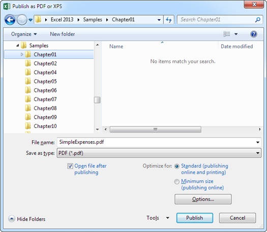
Figure 1-25. You can save PDF files at different resolutions and quality settings (which mostly affect graphics in your workbook, like pictures and charts). Normally, you use higher-quality settings if you want to print your PDF file, because printers use higher resolutions than computers.
The âPublish as PDFâ window gives you some control over the quality of your printout using the âOptimize forâ options. If youâre just saving a PDF copy so other people can view your workbook, choose âMinimum size (publishing online)â to cut down on the storage space required. On the other hand, if people reading your PDF might want to print it out, choose âStandard (publishing online and printing)â to save a slightly larger PDF that makes for a better printout.
You can switch on the âOpen file after publishingâ setting to tell Excel to open the PDF file in Adobe Reader (assuming you have it installed) after it saves the file. That way, you can check the result.
Finally, if you want to publish only a portion of your spreadsheet as a PDF file, click the Options button to open a window with even more settings. You can publish just a fixed number of pages, just selected cells, and so on. These options mirror the choices you see when you print a spreadsheet (Printing). You also see a few more cryptic options, most of which you can safely ignore (theyâre intended for PDF nerds). One exception is the âDocument propertiesâ optionâturn this off if you donât want the PDF to keep track of certain information that identifies you, like your name. (Excel document properties are discussed in more detail on Document Properties.)
Occasionally, you might want to add confidential information to a spreadsheetâa list of the hotels from which youâve stolen spoons, for example. If your computer is on a network, the solution may be as simple as storing your file in the correct, protected location. But if youâre afraid you might email the spreadsheet to the wrong people (say, executives at Four Seasons), or if youâre about to expose systematic accounting irregularities in your companyâs year-end statements, youâll be happy to know that Excel provides a tighter degree of security. It lets you password-protect your spreadsheets, which means that anyone who wants to open them has to know the password you set.
Excel actually has two layers of password protection you can apply to a spreadsheet:
You can prevent others from opening your spreadsheet unless they know the password. This level of security, which scrambles your data for anyone without the password (a process known as encryption), is the strongest.
You can let others read but not modify the sheet unless they know the password.
To apply one or both of these restrictions to your spreadsheet, follow these steps:
Choose FileâSave As, and then choose a location.
The Save As window opens.
From the Tools drop-down menu, pick General Options.
The Tools drop-down menu sits in the bottom-right corner of the Save As window, just to the left of the Save button.
The General Options window appears.
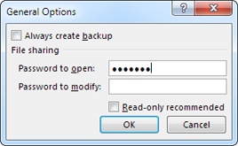
Type a password next to the security level you want to turn on (as shown in Figure 1-26), and then click OK.
The General Options window also gives you a couple of other unrelated options:
Turn on the âAlways create backupâ checkbox if you want a copy of your file in case something goes wrong with the first one (think of it as insurance). Excel creates a backup with the file extension .xlk. For example, if you save a workbook named SimpleExpenses.xlsx with the âAlways create backupâ option on, Excel creates a file named âBackup of SimpleExpenses.xlkâ every time you save your spreadsheet. You can open the .xlk file in Excel just as you would an ordinary Excel file. When you do, you see that it is an exact copy of your work.
Turn on the âRead-only recommendedâ checkbox to prevent other people from accidentally making changes to your spreadsheet. With this option, Excel displays a message every time you (or anyone else) opens the file. It politely suggests that you open the spreadsheet in read-only mode, which means that Excel wonât let you make any changes to the file. Of course, itâs entirely up to the person opening the file whether to accept this recommendation.
If you use a password to restrict people from opening the spreadsheet, Excel prompts you to supply the âpassword to openâ the next time you open the file (Figure 1-27, top).
If you use a password to restrict people from modifying the spreadsheet, the next time you open this file, Excel gives you the choice, shown in Figure 1-27 bottom, to open it in read-only mode (which requires no password) or to open it in full edit mode (in which case youâll need to supply the âpassword to modifyâ).
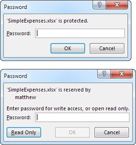
Figure 1-27. Top: You can give a spreadsheet two layers of protection. Assign a âpassword to open,â and youâll see this window when you open the file. Bottom: If you assign a âpassword to modify,â youâll see the choices in this window. If you use both passwords, youâll see both windows, one after the other.
The corollary to the edict âSave your data early and oftenâ is the truism âSometimes things fall apart quicklyâ¦before you even had a chance to back up.â Fortunately, Excel includes an invaluable safety net called AutoRecover.
AutoRecover periodically saves backup copies of your spreadsheet while you work. If you suffer a system crash, you can retrieve the last backup even if you never managed to save the file yourself. Of course, even the AutoRecover backup wonât necessarily have all the information you entered in your spreadsheet before the problem occurred. But if AutoRecover saves a backup every 10 minutes (the standard), at most youâll lose 10 minutesâ worth of work.
If your computer does crash, when you get it running again, you can easily retrieve your last AutoRecover backup. In fact, the next time you launch Excel, it automatically checks the backup folder and, if it finds a backup, it adds a link named Show Recovered Files to Excelâs welcome page (Figure 1-28). Click that link, and Excel adds a panel named Document Recovery to the left side of the Excel window (Figure 1-29).
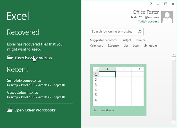
Figure 1-28. Excelâs got your backâclick Show Recovered Files to see what files itâs rescued.
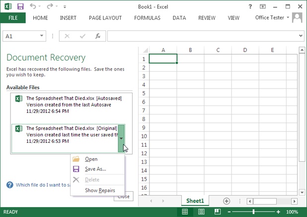
Figure 1-29. You can save or open an AutoRecover backup just as you would an ordinary Excel file; simply click the item in the list. Once you deal with all the backup files, close the Document Recovery window by clicking the Close button. If you havenât saved the backup, Excel asks you whether you want to save it permanently or delete it.
If your computer crashes mid-edit, the next time you open Excel you may see the same file listed twice in the Document Recovery window, as shown in Figure 1-29. The difference is in the status: â[Autosaved]â indicates the most recent backup Excel created, while â[Original]â means the last version of the file you saved (which is safely stored on your hard drive, right where you expect it).
To open a file in the Document Recovery window, just click it. You can also use a drop-down menu with additional options (Figure 1-29). If you find a file you want to keep permanently, make sure to save it. If you donât, the next time you close Excel it asks if it should throw the backups away.
If you attempt to open a backup file thatâs somehow been scrambled (technically known as corrupted), Excel attempts to repair it. You can choose Show Repairs to display a list of any changes Excel made to recover the file.
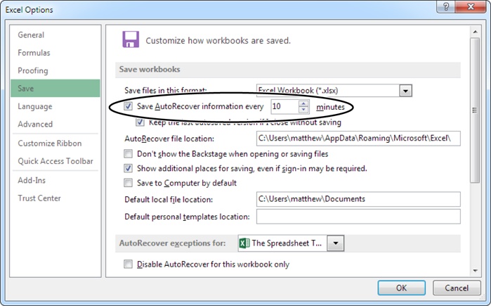
AutoRecover comes switched on when you install Excel, but you can tweak its settings. Choose FileâOptions, and then choose the Save section. Under the âSave workbooksâ section, make sure you have âSave AutoRecover informationâ turned on.
You can make a few other changes to AutoRecover:
You can adjust the backup frequency in minutes. (See Figure 1-30 for tips on timing.)
You can control whether Excel keeps a backup if you create a new spreadsheet, work on it for at least 10 minutes, and then close it without saving your work. This sort of AutoRecover backup is called a draft, and itâs discussed in more detail on AutoRecover. Ordinarily, the setting âKeep the last Auto Recovered file if I exit without savingâ is switched on, and Excel keeps drafts. (To find all the drafts that Excel has saved for you, choose FileâOpen, and scroll to the end of the list of recently opened workbooks, until you see the Recover Unsaved Workbooks button. Click it.)
Figure 1-30. You can configure how often AutoRecover backs up your files. Thereâs really no danger in being too frequent. Unless you work with extremely complex or large spreadsheetsâwhich might suck up a lot of computing power and take a long time to saveâyou can set Excel to save a document every 5 minutes with no appreciable slowdown in performance.
You can choose where you want Excel to save backup files. The standard folder works fine for most people, but feel free to pick some other place. Unfortunately, thereâs no handy Browse button to help you locate the folder, so you need to find the folder in advance (using a tool like Windows Explorer), write it down somewhere, and then copy the full folder path into this window.
Under the âAutoRecover exceptionsâ heading, you can tell Excel not to bother saving a backup of a specific spreadsheet. Pick the spreadsheet name from the list (which shows all the currently open spreadsheet files), and then turn on the âDisable AutoRecover for this workbook onlyâ setting. This setting is exceedingly uncommon, but you might use it if you have a gargantuan spreadsheet full of data that doesnât need to be backed up. For example, this spreadsheet might hold records you pulled out of a central database so you can take a closer look. In such a case, you donât need to create a backup because your spreadsheet is just a copy of the data in the database. (If youâre interested in learning more about this scenario, check out Chapter 27.)
To open files in Excel, you begin by choosing FileâOpen (or using the keyboard shortcut Ctrl+O). This takes you to the Open page in Excelâs backstage view. The left side of the page includes the Places list, which matches the list in the Save As page with one addition: Recent Workbooks. Click this, and youâll see up to 25 of the most recent spreadsheet files you worked on. If you find the file you want, click it to open it.
Note
When you open a file, Excel loads it into a new window. If you already have a workbook on the go, that workbook remains open in a separate Excel window.
The best part about the Recent Documents list is the way you can pin a document so it stays there forever, as shown in Figure 1-31.
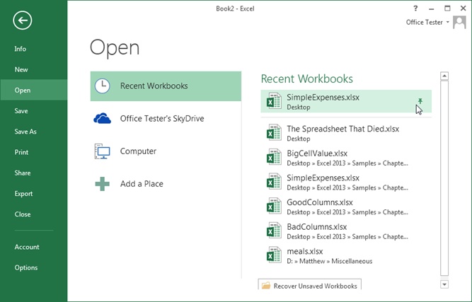
Figure 1-31. To keep a spreadsheet on the Recent Documents list, click the thumbtack on the right. Excel moves your workbook to the top of the list and pins it in place. That means it wonât ever leave the list, no matter how many documents you open. If you decide to stop working with the file later on, just click the thumbtack again to release it. Pinning is a great way to keep your most important files at your fingertips.
Tip
Do you want to hide your recent editing work? You can remove any file from the recent document list by right-clicking it and choosing âRemove from list.â And if the clutter is keeping you from finding the workbooks you want, pin the important files, then right-click any file and choose âClear unpinned workbooks.â This action removes every file that isnât pinned down.
If you donât see the file you want in the list of recent workbooks, you can choose one of the other locations in the Places list. Choose Computer to see a list of locations on your hard drive.
As with recently opened workbooks, you can pin your favorite locations so they remain on this list permanently. To open a file in one of these locations, click the folder (or click the Browse button underneath to look somewhere else). Either way, Excel opens the familiar Open window, where you can pick the file you want.
Tip
The Open window also lets you open several spreadsheets in one step, as long as theyâre all in the same folder. To use this trick, hold down the Ctrl key and click to select each file. When you click Open, Excel puts each one in a separate window, just as if youâd opened them one after the other.
Excel can open many file types other than its native .xlsx format. To open files in another format, begin by choosing FileâOpen, and then pick a location. When the Open window appears, pick the type of format you want from the âFiles of typeâ list at the bottom.
If you want to open a file but donât know what format itâs in, try using the first option in the list, âAll Files.â Once you choose a file, Excel scans the beginning of the file and informs you about the type of conversion it will attempt (based on the type of file Excel thinks it is).
Note
Depending on your computer settings, Windows might hide file extensions. That means that instead of seeing the Excel spreadsheet file MyCoalMiningFortune.xlsx, youâll just see the name MyCoalMiningFortune (without the .xlsx part on the end). In this case, you can still tell what type of file it is by looking at the icon. If you see a small Excel icon next to the file name, that means Windows recognizes the file as an Excel spreadsheet. If you see something else (like a tiny paint palette, for example), you need to make a logical guess as to what type of file it is.
Even something that seems as innocent as an Excel file canât always be trusted. Protected view is an Excel security feature that aims to keep you safe. It opens potentially risky Excel files in a specially limited Excel window. Youâll know youâre in protected view because Excel doesnât let you edit any of the data in the workbook, and it displays a message bar at the top of the window (Figure 1-32).
Excel automatically uses protected view when you download a spreadsheet from the Web or open it from your email inbox. This is actually a huge convenience, because Excel doesnât need to hassle you with questions when you try to view the file (such as âAre you sure you want to open this file?â). Because Excelâs protected view has bullet-proof security, itâs a safe way to view even the most suspicious spreadsheet.

Figure 1-32. Currently, this file is in protected view. If you decide that itâs safe and you need to edit its content, click the Enable Editing button to open the file in the normal Excel window with no security safeguards.
At this point, youâre probably wondering about the risks of rogue spreadsheets. Truthfully, theyâre quite small. The most obvious danger is macro code: miniature programs stored in a spreadsheet file that perform Excel tasks. Poorly written or malicious macro code can tamper with your Excel settings, lock up the program, and even scramble your data. But before you panic, consider this: Excel macro viruses are very rare, and the .xlsx file format doesnât even allow macro code. Instead, macro-containing files must be saved as .xlsm or .xlsb files.
The more subtle danger here is that crafty hackers could create corrupted Excel files that might exploit tiny security holes in the program. One of these files could scramble Excelâs brains in a dangerous way, possibly causing it to execute a scrap of malicious computer code that could do almost anything. Once again, this sort of attack is extremely rare. It might not even be possible with the up-to-date .xlsx file format. But protected view completely removes any chance of an attack, which helps corporate bigwigs sleep at night.
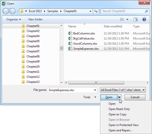
The Open window harbors a few tricks. To see these hidden secrets, first select the file you want to use (by clicking it once, not twice), and then click the drop-down arrow on the right-side of the Open button. A menu with several options appears, as shown in Figure 1-33.
Hereâs what these different choices do:
Open opens the file in the normal way.
Open Read-Only opens the file, but wonât let you save changes. This option is great if you want to make sure you donât accidentally overwrite an existing file. (For example, if youâre using last monthâs sales invoice as a starting point for this monthâs invoice, you might use Open Read-Only to make sure you canât accidentally wipe out the existing file.) If you open a document in read-only mode, you can still make changesâyou just have to save the file with a new file name (choose FileâSave As).
Open as Copy creates a copy of the spreadsheet in the same folder. If you named your file Book1.xlsx, the copy will be named Copy of Book1.xlsx. This feature comes in handy if youâre about to start editing a spreadsheet and want to be able to look at the last version you saved. Excel wonât let you open the same file twice, but you can load the previous version by selecting the same file and using âOpen as Copy.â (Of course, this technique works only when you have changes you havenât saved yet. Once you save the current version of a file, Excel overwrites the older version and itâs lost forever.)
Open in Browser is only available when you select an HTML file. This option lets you open the HTML file in your computerâs web browser. Itâs part of an old Excel feature that allows you to save spreadsheets as web pages, which has now been replaced by Excelâs Web App (Putting Your Files Online).
Open in Protected View prevents a potentially dangerous file from running any code. However, youâll also be restrained from editing the file, as explained on Opening Files in Other Formats.
Open and Repair is useful if you need to open a file thatâs corrupted. If you try to open a corrupted file by just clicking Open, Excel warns you that the file has problems and refuses to open it. To get around this, you can open the file using the âOpen and Repairâ option, which prompts Excel to make the necessary corrections, display them for you in a list, and then open the document. Depending on the type of problem, you might not lose any information at all.
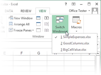
As you open multiple spreadsheets, Excel creates a new window for each one. Although this helps keep your work separated, it can cause a bit of clutter and make it harder to track down the window you really want. Fortunately, Excel provides a few shortcuts that are indispensable when dealing with several spreadsheets at a time:
To jump from one spreadsheet to another, find the window in the ViewâWindowâSwitch Windows list, which includes the file name of all the currently open spreadsheets (Figure 1-34).
To move to the next spreadsheet, use the keyboard shortcut Ctrl+Tab or Ctrl+F6.
To move to the previous spreadsheet, use the shortcut key Ctrl+Shift+Tab or Ctrl+Shift+F6.
Note
One of the weirdest limitations in Excel occurs if you try to open more than one file with the same name. No matter what steps you take, you canât coax Excel to open both of them at once. It doesnât matter if the files have different content or if theyâre in different folders or even on different drives. When you try to open a file that has the same name as a file thatâs already open, Excel displays an error message and refuses to go any further. Sadly, the only solution is to open the files one at a time, or rename one of them.
Get Excel 2013: The Missing Manual now with the O’Reilly learning platform.
O’Reilly members experience books, live events, courses curated by job role, and more from O’Reilly and nearly 200 top publishers.

