Every Excel grandmaster needs to start somewhere. In this chapter, you’ll learn how to create a basic spreadsheet. First, you’ll learn to move around Excel’s grid of cells, typing in numbers and text as you go. Next, you’ll take a quick tour of the Excel window, stopping to meet the different tabs in the ribbon and take a quick peek at the formula bar. Finally, you’ll get a tour of Excel’s innovative backstage view—the file-management hub where you can save your work for posterity, open recent files, and tweak Excel options.
Note
Even if you’re an Excel old-timer, don’t bypass this chapter. Although you already know how to fill in a simple spreadsheet, you haven’t seen Excel’s backstage view, which is a completely new feature in Excel 2010. It gives you a single, streamlined place to perform a whole variety of tasks, most of which have to do with managing your files. To skip the review and pick up your backstage pass, jump straight to Going Backstage.
When you first launch Excel, it starts you off with a new, blank worksheet, as shown in Figure 1-1. A worksheet is the grid of cells where you type your information and formulas. This grid takes up most of the Excel window. It’s where you’ll perform all your work, such as entering data, writing formulas, and reviewing the results.
Here are a few basics about Excel’s grid:
The grid divides your worksheet into rows and columns. Columns are identified with letters (A, B, C…), while rows are identified with numbers (1, 2, 3…).
The smallest unit in your worksheet is the cell. Cells are identified by column and row. For example, C6 is the address of a cell in column C (the third column) and row 6 (the sixth row). Figure 1-2 shows this cell, which looks like a rectangular box. Incidentally, an Excel cell can hold up to 32,000 characters.
A worksheet can span an eye-popping 16,000 columns and 1 million rows. In the unlikely case that you want to go beyond those limits—say, if you’re tracking blades of grass on the White House lawn—you’ll need to create a new worksheet. Every spreadsheet file can hold a virtually unlimited number of worksheets, as you’ll learn in Chapter 4.
When you enter information, enter it one cell at a time. However, you don’t have to follow any set order. For example, you can start by typing information into cell A40 without worrying about filling any data in the cells that appear in the earlier rows.
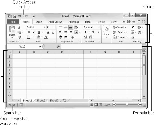
Figure 1-1. The largest part of the Excel window is the worksheet grid, where you type in your information.
Note
Obviously, once you go beyond 26 columns, you run out of letters. Excel handles this by doubling up (and then tripling up) letters. For example, column Z is followed by column AA, then AB, then AC, all the way to AZ and then BA, BB, BC—you get the picture. And if you create a ridiculously large worksheet, you’ll find that column ZZ is followed by AAA, AAB, AAC, and so on.

Figure 1-2. Here, the current cell is C6. You can recognize the current (or active) cell based on its heavy black border. You’ll also notice that the corresponding column letter (C) and row number (6) are highlighted at the edges of the worksheet. Just above the worksheet, on the left side of the window, the formula bar tells you the active cell address.
The best way to get a feel for Excel is to dive right in and start putting together a worksheet. The following sections cover each step that goes into assembling a simple worksheet. This one tracks household expenses, but you can use the same approach to create any basic worksheet.
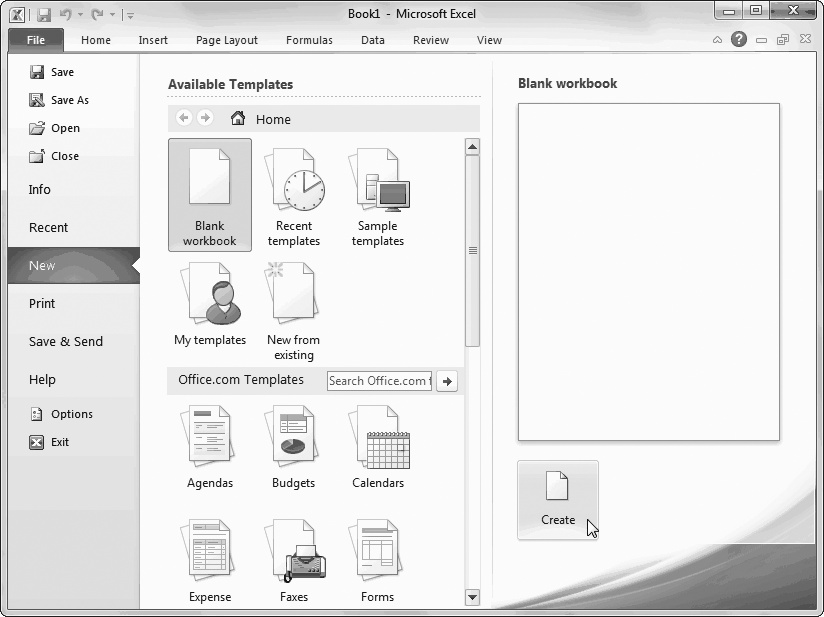
When you fire up Excel, it opens a fresh workbook file. If you’ve already got Excel open and you want to create another workbook, just choose File→New (where File switches you into Excel’s backstage view, and New is a command on the left side of the window). You’ll see a variety of options for creating specialized types of spreadsheets. But to get started with a blank canvas, keep “Blank workbook” selected and click the Create button, as shown in Figure 1-3.
Note
A workbook is a collection of one or more worksheets. That distinction isn’t terribly important now because you’re using only a single worksheet in each workbook you create. But in Chapter 4, you’ll learn how to use several worksheets in the same workbook to track related collections of data.
For now, all you need to know is that the worksheet is the grid of cells where you place your data, and the workbook is the spreadsheet file that you save on your computer.
You don’t need to pick the file name for your workbook when you first create it. Instead, that decision happens later, when you save your workbook. For now, you start with a blank canvas that’s ready to receive your numerical insights.
Note
Creating new workbooks doesn’t disturb what you’ve already done. Whatever workbook you were using remains open in another window. You can use the taskbar to move from one workbook to the other, or you can use the Excel shortcuts explained on Working with Multiple Open Spreadsheets.
Excel allows you to arrange information in whatever way you like. There’s nothing to stop you from scattering numbers left and right, across as many cells as you can. However, one of the most common (and most useful) ways to arrange your information is as a table, with headings for each column.
It’s important to remember that even for the simplest worksheet, the decisions you make about what’s going to go in each column can have a big effect on how easy it is to manipulate your information. For example, in a worksheet that stores a mailing list, you could have two columns: one for names and another for addresses. But if you create more than two columns, your life will probably be easier since you can separate first names from street addresses from ZIP codes, and so on. Figure 1-4 shows the difference.
You can, of course, always add or remove columns later. But you can avoid getting gray hairs by starting a worksheet with all the columns you think you’ll need.
The first step in creating your worksheet is to add your headings in the row of cells at the top of the worksheet (row 1). Technically, you don’t need to start right in the first row, but unless you want to add more information before your table—like a title for the chart or today’s date—there’s no point in wasting the space. Adding information is easy—just click the cell you want and start typing. When you’re finished, hit Tab to complete your entry and move to the next cell to the right (or Enter to head to the cell just underneath).
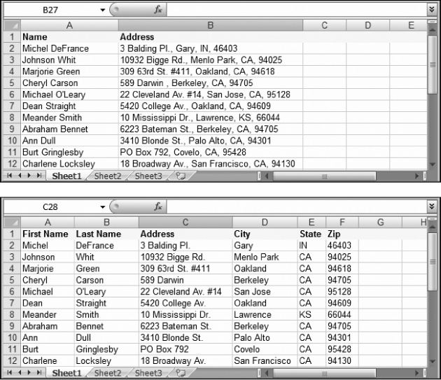
Figure 1-4. Top: If you enter the first and last names together in one column, Excel can sort only by the first names. And if you clump the addresses and ZIP codes together, you give Excel no way to count how many people live in a certain town or neighborhood, because Excel can’t extract the ZIP codes. Bottom: The benefit of a six-column table is significant: It lets you sort (reorganize) your list according to people’s last names or where they live. It also allows you to filter out individual bits of information when you start using functions later in this book.
Note
The information you put in an Excel worksheet doesn’t need to be in neat, ordered columns. Nothing stops you from scattering numbers and text in random cells. However, most Excel worksheets resemble some sort of table, because that’s the easiest and most effective way to deal with large amounts of structured information.
For a simple expense worksheet designed to keep a record of your most prudent and extravagant purchases, try the following three headings:
Date Purchased stores the date when you spent the money.
Item stores the name of the product that you bought.
Price records how much it cost.
Right away, you face your first glitch: awkwardly crowded text. Figure 1-5 shows how you can adjust column width for proper breathing room.
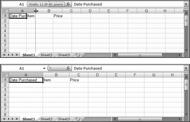
Figure 1-5. Top: The standard width of an Excel column is 8.43 characters, which hardly allows you to get a word in edgewise. To solve this problem, position your mouse on the right border of the column header you want to expand so that the mouse pointer changes to the resize icon (it looks like a double-headed arrow). Now drag the column border to the right as far as you want. As you drag, a tooltip appears, telling you the character size and pixel width of the column. Both of these pieces of information play the same role—they tell you how wide the column is—only the unit of measurement changes. Bottom: When you release the mouse, the entire column of cells is resized to the new size.
Note
A column’s character width doesn’t really reflect how many characters (or letters) fit in a cell. Excel uses proportional fonts, in which different letters take up different amounts of room. For example, the letter W is typically much wider than the letter 1. All this means is that the character width Excel shows you isn’t a real indication of how many letters can fit in the column, but it’s still a useful measurement that you can use to compare different columns.
You can now begin adding your data: simply fill in the rows under the column titles. Each row in the expense worksheet represents a separate purchase you’ve made. (If you’re familiar with databases, you can think of each row as a separate record.)
As Figure 1-6 shows, the first column is for dates, the second column is for text, and the third column holds numbers. Keep in mind that Excel doesn’t impose any rules on what you type, so you’re free to put text in the Price column. But if you don’t keep a consistent kind of data in each column, you won’t be able to easily analyze (or understand) your information later.
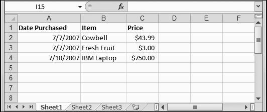
Figure 1-6. This rudimentary expense list has three items (in rows 2, 3, and 4). The alignment of each column reflects the data type (by default, numbers and dates are right-aligned, while text is left-aligned), indicating that Excel understands your date and price information.
That’s it. You’ve now created a living, breathing worksheet. The next section explains how you can edit the data you’ve entered.
Every time you start typing in a cell, Excel erases any existing content in that cell. (You can also quickly remove the contents of a cell by just moving to it and pressing Delete, which clears its contents.)
If you want to edit cell data instead of replacing it, you need to put the cell in edit mode, like this:
Move to the cell you want to edit.
Use the mouse or the arrow keys to get to the correct cell.
Put the cell in edit mode by pressing F2.
Edit mode looks almost the same as ordinary text entry mode. The only difference is that you can use the arrow keys to move through the text you’re typing and make changes. (When you aren’t in edit mode, pressing these keys just moves you to another cell.)
If you don’t want to use F2, you can also get a cell into edit mode by double-clicking it.
Complete your edit.
Once you’ve modified the cell content, press Enter to make your change or Esc to cancel your edit and leave the old value in the cell. Alternatively, you can click on another cell to accept the current value and go somewhere else. But while you’re in edit mode, you can’t use the arrow keys to move out of the cell.
Tip
If you start typing new information into a cell and you decide you want to move to an earlier position in your entry (to make an alteration, for instance), just press F2. The cell box still looks the same, but you’re now in edit mode, which means that you can use the arrow keys to move within the cell (instead of moving from cell to cell). You can press F2 again to return to the normal data entry mode, which allows you to use the arrow keys to move to another cell.
As you enter data, you may discover the Bigtime Excel Display Problem (known to aficionados as BEDP): Cells in adjacent columns can overlap one another. Figure 1-7 shows the problem. One way to fix BEDP is to manually resize the column, as shown in Figure 1-5. Another option is to use wrapping to fit multiple lines of text in a single cell, as described on Alignment and Orientation.
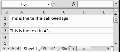
Figure 1-7. Overlapping cells can create big headaches. For example, if you type a large amount of text into A1, and then you type some text into B1, you see only part of the data in A1 on your worksheet (as shown here). The rest is hidden from view. But if, say, A3 contains a large amount of text and B3 is empty, the content in A3 is displayed over both columns, and you don’t have a problem.
Learning how to move around the Excel grid quickly and confidently is an indispensable skill. To move from cell to cell, you have two fairly obvious choices:
Use the arrow keys on the keyboard. Keystrokes move you one cell at a time in any direction.
Click the cell with the mouse. A mouse click jumps you directly to the cell you’ve clicked.
As you move from cell to cell, you see the black focus box move to highlight the currently active cell.
In some cases, you might want to cover ground a little quicker. One option is to use the scrollbars at the bottom and on the right side of the window to scroll off into the uncharted regions of your worksheet. Excel also provides two more powerful features—shortcut keys and the Go To feature—which are described in the following sections.
Excel provides a number of handy key combinations that can transport you across your worksheet in great leaps and bounds (see Table 1-1). The most useful shortcut keys include the Home key combinations, which bring you back to the beginning of a row or the top of your worksheet.
Note
Shortcut key combinations that use the + sign must be entered together. For example, “Ctrl+Home” means you hold down Ctrl and press Home at the same time. Key combinations with a comma work in sequence. For example, the key combination “End, Home” means press End first, release it, and then press Home.
Table 1-1. Shortcut keys for moving around a worksheet
Excel also lets you cross great distances in a single bound using a Ctrl+arrow key combination. These key combinations jump to the edges of your data. Edge cells include cells that are next to other blank cells. For example, if you press Ctrl+→ while you’re inside a group of cells with information in them, you’ll skip to the right, over all filled cells, and stop just before the next blank cell. If you press Ctrl+→ again, you’ll skip over all the nearby blank cells and land in the next cell to the right that has information in it. If there aren’t any more cells with data on the right, you’ll wind up on the very edge of your worksheet.
The Ctrl+arrow key combinations are useful if you have more than one table of data in the same worksheet. For example, imagine you have two tables of data, one at the top of a worksheet and one at the bottom. If you are at the top of the first table, you can use Ctrl+↓ to jump to the bottom of the first table, skipping all the rows in between. Press Ctrl+↓ again, and you leap over all the blank rows, winding up at the beginning of the second table.
If you’re fortunate enough to know exactly where you need to go, you can use the Go To feature to make the jump. Go To moves to the cell address you specify. It comes in useful in extremely large spreadsheets, where just scrolling through the worksheet takes half a day.
To bring up the Go To dialog box (shown in Figure 1-8), choose Home→Editing→Find & Select→Go To. Or you can do yourself a favor and just press Ctrl+G. Enter the cell address (such as C32), and then click OK.
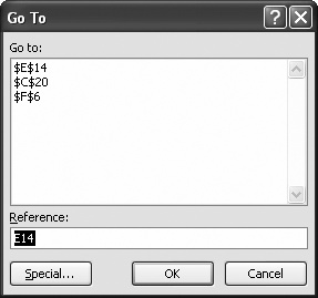
Figure 1-8. You’ll notice that in the Go To list, cell addresses are written a little differently than the format you use when you type them in. Namely, dollar signs are added before the row number and column letter. Thus, C32 becomes $C$32, which is simply the convention that Excel uses for fixed cell references. (You’ll learn much more about the different types of cell references in Chapter 8.)
The Go To feature becomes more useful the more you use it. That’s because the Go To window maintains a list of the most recent cell addresses that you’ve entered. In addition, every time you open the Go To window, Excel automatically adds the current cell to the list. This feature makes it easy to jump to a far-off cell and quickly return to your starting location by selecting the last entry in the list.
The Go To window isn’t your only option for leaping through a worksheet in a single bound. If you look at the Home→Editing→Find & Select menu, you’ll find more specialized commands that let you jump straight to cells that contains formulas, comments, conditional formatting, and other advanced Excel ingredients that you haven’t learned about yet. And if you want to hunt down cells that have specific text, you need the popular Find command (Home→Editing→Find & Select→Find), which is covered on Entering data in grouped sheets.
Finding your way around a worksheet is a fundamental part of mastering Excel. Knowing your way around the larger program window is no less important. The next few sections help you get oriented in the Excel window, pointing out the important stuff and letting you know what you can usually ignore.
In the Introduction, you learned about the ribbon, the super-toolbar that offers one-stop shopping for all of Excel’s features. All the most important Office applications—including Word, Access, PowerPoint, and Excel—use the ribbon. However, each program has a different set of tabs and buttons.
Throughout this book, you’ll dig through the different tabs of the ribbon to find important features. But before you start your journey, it’s nice to get a quick overview of what each tab provides. Here’s the lowdown:
File isn’t really a toolbar tab, even though it appears first in the list. Instead, it’s your gateway to Excel’s backstage view, as described on Going Backstage.
Home includes some of the most commonly used buttons, like those for cutting and pasting information, formatting your data, and hunting down important bits of information with search tools. You’ve already used the Go To button on this tab (see page The Go To Feature).
Insert lets you add special ingredients like tables, graphics, charts, and hyperlinks.
Page Layout is all about getting your worksheet ready for the printer. You can tweak margins, paper orientation, and other page settings.
Formulas are mathematical instructions that you use to perform calculations. This tab helps you build super-smart formulas and resolve mind-bending errors.
Data lets you get information from an outside data source (like a heavy-duty database) so you can analyze it in Excel. It also includes tools for dealing with large amounts of information, like sorting, filtering, and subgrouping.
Review includes the familiar Office proofing tools (like the spell checker). It also has buttons that let you add comments to a worksheet and manage revisions.
View lets you switch on and off a variety of viewing options. It also lets you pull off a few fancy tricks if you want to view several separate Excel spreadsheet files at the same time.
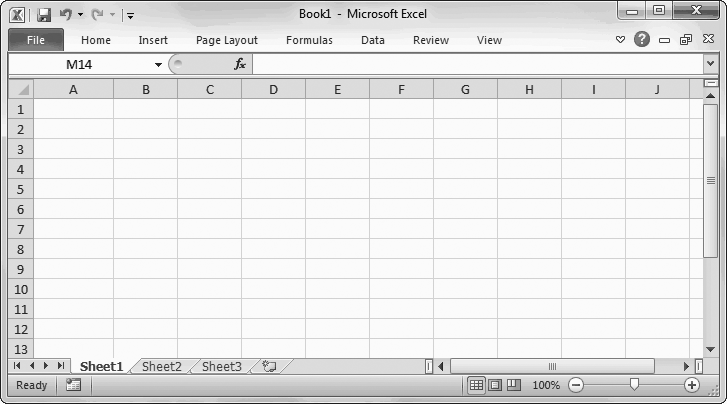
Figure 1-9. Do you want to use every square inch of screen space for your cells? You can collapse the ribbon (as shown here) by double-clicking any tab. Click a tab to pop it open temporarily, or double-click a tab to bring the ribbon back for good. And if you want to perform the same trick without raising your fingers from the keyboard, you can use the shortcut key Ctrl+F1.
Note
In some circumstances, you may see tabs that aren’t listed here. Macro programmers and other highly technical types use the Developer tab. (You’ll learn how to reveal this tab on Attaching a Macro to a Button Inside a Worksheet.) The Add-Ins tab appears when you’re viewing workbooks that were created in previous versions of Excel and used custom toolbars. And finally, you can create a tab of your own if you’re ambitious enough to customize the ribbon, as explained in the appendix.
The formula bar appears above the worksheet grid but below the ribbon (Figure 1-10). It displays the address of the active cell (like A1) on the left edge, and it also shows you the current cell’s contents.
You can use the formula bar to enter and edit data, instead of editing directly in your worksheet. This approach is particularly useful when a cell contains a formula or a large amount of information. That’s because the formula bar gives you more work room than a typical cell. Just as with in-cell edits, you press Enter to confirm your changes or Esc to cancel them. Or you can use the mouse: When you start tying in the formula bar, a checkmark and an “X” icon appear just to the left of the box where you’re typing. Click the checkmark to confirm your entry or “X” to roll it back.
Note
You can hide (or show) the formula bar by choosing View→Show→Formula Bar. But the formula bar is such a basic part of Excel that you’d be unwise to get rid of it. Instead, keep it around until Chapter 8, when you’ll learn how to build formulas.
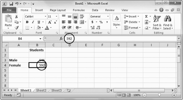
Figure 1-10. The formula bar (just above the grid) shows information about the active cell. In this example, the formula bar shows that the current cell is B4 and that it contains the number 592. Instead of editing this value in the worksheet, you can click anywhere in the formula bar and make your changes there.
Ordinarily, the formula bar is a single line. If you have a really long entry in a cell (like a paragraph’s worth of text), you need to scroll from one side to the other. However, there’s another option—you can resize the formula bar so it fits more information, as shown in Figure 1-11.
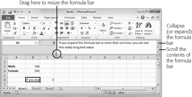
Figure 1-11. To enlarge the formula bar, click the bottom edge and pull down. You can make it two, three, four, or many more lines large. Best of all, once you get the size you want, you can use the expand/collapse button on the right side of the formula bar to quickly expand it to your preferred size and collapse it back to the single-line view.
Though people often overlook it, the status bar (Figure 1-12) is a good way to keep on top of Excel’s current state. For example, if you save or print a document, the status bar shows the progress of the printing process. If you’re performing a quick action, the progress indicator may disappear before you have a chance to even notice it. But if you’re performing a time-consuming operation—say, printing out an 87-page table of the airline silverware you happen to own—you can look to the status bar to see how things are coming along.
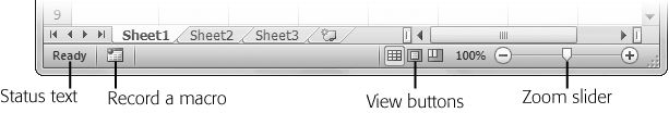
Figure 1-12. In the status bar, you can see the basic status text (which just says “Ready” in this example), the view buttons (which are useful when you’re preparing a spreadsheet for printing), and the zoom slider bar (which lets you enlarge or shrink the current worksheet view).
The status bar combines several different types of information. The leftmost part of the status bar shows the Cell Mode, which displays one of three indicators:
The word “Ready” means that Excel isn’t doing anything much at the moment, other than waiting for you to take some action.
The word “Enter” appears when you start typing a new value into a cell.
The word “Edit” means the cell is currently in edit mode, and pressing the left and right arrow keys moves through the cell data, instead of moving from cell to cell. You can place a cell in edit mode or take it out of edit mode by pressing F2.
Just to the right of the Cell Mode information, you may see a small button that lets you start recording a macro. (A macro is a series of steps you can replay as often as you need to automate tiresome chores. You’ll learn more about macros in Chapter 28.)
Farther to the right on the status bar are the view buttons, which let you switch to Page Layout View or Page Break Preview. These different views help you see what your worksheet will look like when you print it. They’re covered in Chapter 7.
The zoom slider is next to the view buttons, at the far right edge of the status bar. You can slide it to the left to zoom out (which fits more information into your Excel window at once) or slide it to the right to zoom in (and take a closer look at fewer cells). You can learn more about zooming on Zooming.
In addition, the status bar displays other miscellaneous indicators. For example, if you press the Scroll Lock key, a Scroll Lock indicator appears on the status bar (next to the “Ready” text). This indicator tells you that you’re in scroll mode. In scroll mode, the arrow keys don’t move you from one cell to another; instead, they scroll the entire worksheet up, down, or to the side. Scroll mode is a great way to check out another part of your spreadsheet without leaving your current position.
You can control what indicators appear in the status bar by configuring it. To see a full list of possibilities, right-click the status bar. A huge list of options appears, as shown in Figure 1-13. Table 1-2 describes the different status bar options.
Note
The Caps Lock indicator doesn’t determine whether you can use the Caps Lock key—that feature always works. The Caps Lock indicator just lets you know when Caps Lock mode is on. That way you won’t be surprised by an accidental keystroke that turns your next data entry INTO ALL CAPITALS.
Table 1-2. Status bar indicators
Indicator | Meaning |
|---|---|
Cell Mode | Shows Ready, Edit, or Enter depending on the state of the current cell. |
Signatures, Information Management Policy, and Permissions | Displays information about the rights and restrictions of the current spreadsheet. These features come into play only if you’re using Office SharePoint Server to share spreadsheets among groups of people (usually in a corporate environment). SharePoint is introduced on Workbook Sharing in Action. |
Caps Lock | Indicates whether Caps Lock mode is on. When Caps Lock is on, every letter you type is automatically capitalized. To turn Caps Lock mode on or off, hit Caps Lock. |
Num Lock | Indicates whether Num Lock mode is on. When this mode is on, you can use the numeric keypad (typically at the right side of your keyboard) to type in numbers more quickly. When this sign’s off, the numeric keypad controls cell navigation instead. To turn Num Lock on or off, press Num Lock. |
Scroll Lock | Indicates whether Scroll Lock mode is on. When it’s on, you can use the arrow keys to scroll through the worksheet without changing the active cell. (In other words, you can control your scrollbars by just using your keyboard.) This feature lets you look at all the information you have in your worksheet without losing track of the cell you’re currently in. You can turn Scroll Lock mode on or off by pressing Scroll Lock. |
Fixed Decimal | Indicates when Fixed Decimal mode is on. When this mode is on, Excel automatically adds a set number of decimal places to the values you enter in any cell. For example, if you set Excel to use two fixed decimal places and you type the number 5 into a cell, Excel actually enters 0.05. This seldom-used featured is handy for speed typists who need to enter reams of data in a fixed format. You can turn this feature on or off by selecting File®Options, choosing the Advanced section, and then looking under “Editing options” to find the “Automatically insert a decimal point” setting. Once you turn this checkbox on, you can choose the number of decimal places (the standard option is 2). |
Overtype Mode | Indicates when Overwrite mode is turned on. Overwrite mode changes how cell edits work. When you edit a cell and Overwrite mode is on, the new characters that you type overwrite existing characters (rather than displacing them). You can turn Overwrite mode on or off by pressing Insert. |
End Mode | Indicates that you’ve pressed End, which is the first key in many two-key combinations; the next key determines what happens. For example, hit End and then Home to move to the bottom-right cell in your worksheet. See Table 1-1 for a list of key combinations, some of which use End. |
Macro Recording | Macros are automated routines that perform some task in an Excel spreadsheet. The Macro Recording indicator shows a record button (which looks like a red circle superimposed on a worksheet) that lets you start recording a new macro. You’ll learn more about macros in Chapter 28. |
Selection Mode | Indicates the current Selection mode. You have two options: normal mode and extended selection. When you press the arrows keys and extended selection is on, Excel automatically selects all the rows and columns you cross. Extended selection is a useful keyboard alternative to dragging your mouse to select swaths of the grid. To turn extended selection on or off, press F8. You’ll learn more about selecting cells and moving them around in Chapter 3. |
Page Number | Shows the current page and the total number of pages (as in "The Missing Manual Series of 4”). This indicator appears only in Page Layout view (as described on Page Layout View: A Better Print Preview). |
Average, Count, Numerical Count, Minimum, Maximum, Sum | Show the result of a calculation on the selected cells. For example, the Sum indicator shows the total of all the numeric cells that are currently selected. You’ll take a closer look at this handy trick on Making Continuous Range Selections. |
Upload Status | Does nothing (that we know of). Excel does show a handy indicator in the status bar when you’re uploading files to the Web, as you’ll learn in Chapter 26. However, the upload status is always shown, and this setting doesn’t seem to have any effect. |
View Shortcuts | Shows the three view buttons that let you switch between Normal view, Page Layout View, and Page Break Preview. |
Zoom | Shows the current zoom percentage (like 100 percent for a normal-sized spreadsheet, and 200 percent for a spreadsheet that’s blown up to twice the magnification). |
Zoom Slider | Shows a slider that lets you zoom in closer (by sliding it to the right) or out to see more information at once (by sliding it to the left). |
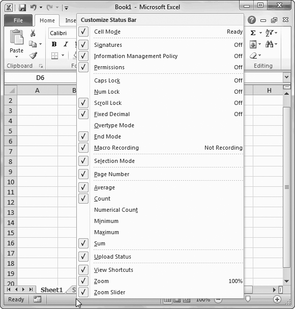
Figure 1-13. Every item that has a checkmark appears in the status bar when you need it. For example, if you choose Caps Lock, the text “Caps Lock” appears in the status bar whenever you hit the Caps Lock key to switch to all-capital typing. The text that appears on the right side of the list tells you the current value of the indicator. In this example, Caps Lock mode is currently off and the Cell Mode text says “Ready.”
Your data is the star of the show. That’s why the creators of Excel refer to your worksheet as being “on stage.” The auditorium is the Excel main window, which—as you’ve just seen—includes the handy ribbon, formula bar, and status bar. Sure, it’s a strange metaphor. But once you understand it, you’ll realize the rationale for Excel’s backstage view, which temporarily takes you away from your worksheet and lets you concentrate on other tasks that don’t involve entering or editing data. These tasks include saving your spreadsheet, opening more spreadsheets, printing your work, and changing Excel settings.
To switch to backstage view, click the File button that’s just to the left of the Home ribbon tab. Excel temporarily tucks your worksheet out of sight (although it’s still open and waiting for you). This gives it space to show extra information related to the task you want to perform, as shown in Figure 1-14. For example, if you plan to print your spreadsheet, Excel’s backstage view has room to show a preview of the printout. Or if you want to open an existing spreadsheet, Excel can show a detailed list of files you’ve recently worked on.
To get out of backstage view and return to your worksheet, just click the File button again, or press Esc.
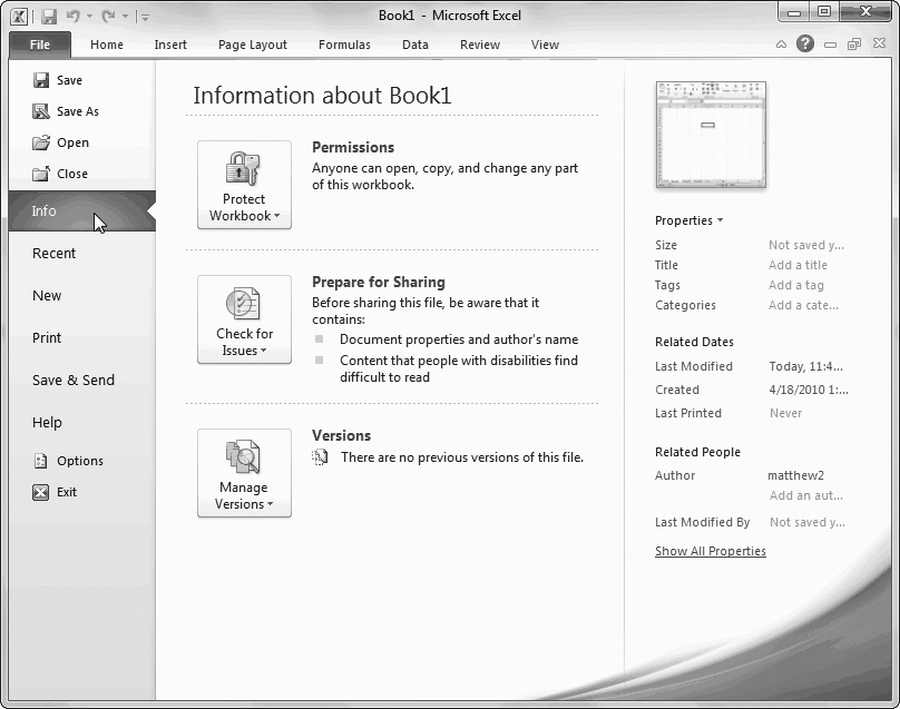
Figure 1-14. When you first switch to backstage view, Excel shows the Info page, which provides some basic information about your workbook file, its size, when it was last edited, who edited it, and so on (see the column on the far right). The Info page also provides the gateway to three important features: document protection (Chapter 24), compatibility checking (page 41), and AutoRecover backups (page 82). To go to another section, click a different command in the column on the far left.
The Excel Options window provides a central hub where you can adjust how Excel looks, behaves, and calculates (see Figure 1-15). To get to this window, choose File→Options.
The various sections in the Excel Options window let you tweak a wide variety of different details. Some of these details are truly handy, like the options for opening and saving files (which are described at the end of this chapter). Others are seldom-used holdovers from the past, like the option that lets Excel act like Lotus—an ancient piece of spreadsheet software—when you hit the “/” key.
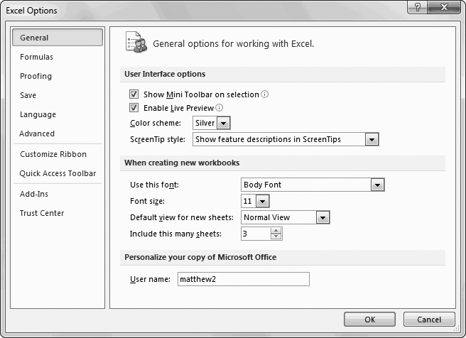
Figure 1-15. The Excel Options window is divided into 10 sections. To pick which section to look at, choose an entry from the list on the left. In this example, you’re looking at the General settings group. In each section, the settings are further subdivided into titled groups. You may need to scroll down to find the setting you want.
Tip
Some important options have a small i-in-a-circle icon next to them, which stands for “information.” Hover over this icon, and you see a tooltip that gives you a brief description about that setting.
While you’re getting to know Excel, you can comfortably ignore most of what’s in the Excel Options window. But you’ll return here many times throughout this book to adjust settings and fine-tune the way Excel works.
As everyone who’s been alive for at least three days knows, you should save your work early and often. Excel is no exception. You have three choices for saving a spreadsheet file:
Save. This action updates the spreadsheet file with your most recent changes. If you use Save on a new file that hasn’t been saved before Excel prompts you to choose a folder and file name. To use Save, select File→Save, or press Ctrl+S. Or look up at the top of the Excel window in the Quick Access toolbar for the tiny Save button, which looks like an old-style diskette.
Save As. This choice allows you to save your spreadsheet file with a new name. You can use Save As the first time you save a new spreadsheet, or you can use it to save a copy of your current spreadsheet with a new name, in a new folder, or as a different file type. To use Save As, select File→Save As, or press F12.
Save & Send. The File→Save & Send page in Excel’s backstage view provides several of the same options you get from the Save As dialog box. The difference is that it makes them a bit more obvious and a bit more convenient. Figure 1-16 shows what to look for.
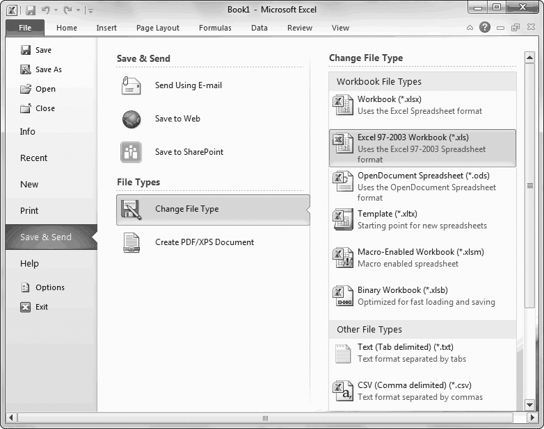
Figure 1-16. Using File→Save & Send, you can email a copy of your workbook (page 723), transfer it to the Excel Web App (Chapter 26), or upload it to SharePoint (page 746). But ignore these options for now and focus on the “File Types” section underneath, which gives you shortcuts for saving your work in alternative file formats. If you click Change File Type, you get a list with the most common file formats (on the right). Double-click an entry to open the Save As dialog box with that selection. Or click Create PDF/XPS Document to create a print-ready PDF document, as described on page 44.
Since time immemorial, Excel fans have been saving their lovingly crafted spreadsheets in .xls files (as in AirlineSilverware.xls). But when Excel 2007 hit the streets, it introduced a completely new file format, with the extension .xlsx (as in AirlineSilverware.xlsx). Excel 2010 keeps the .xlsx revamped format, without introducing any more changes.
As an Excel user, you need to decide whether you want to save your spreadsheets in the latest and greatest .xlsx format or in the older .xls format. But before you make that decision, it helps to know a bit more about the advantages of the .xlsx format:
It’s compact. The .xlsx format uses ZIP file compression, so spreadsheet files are smaller—way smaller (as much as 75 percent smaller than their original sizes). And even though the average hard drive is already large enough to swallow thousands of old-fashioned Excel files, the new compact format is easier to email around.
It’s less error-prone. The .xlsx format carefully separates ordinary content, pictures, and macro code into separate sections. Microsoft claims that this change makes for tougher files. Now, if a part of your Excel file is damaged (for example, due to a faulty hard drive), there’s a much better chance that you can still retrieve the rest of the information. (You’ll learn about Excel disaster recovery on Disaster Recovery.)
It’s extensible. The .xlsx format uses XML (the eXtensible Markup Language), which is a standardized way to store information. (You’ll learn more about XML in Chapter 23.) XML storage doesn’t benefit the average person, but it’s sure to earn a lot of love from companies that plan to build custom software that uses Excel documents. As long as Excel documents are stored in XML, these companies can create automated programs that pull the information they need straight out of a spreadsheet, without going through Excel. These programs can also generate made-to-measure Excel documents all on their own.
For all these reasons, .xlsx is the format of choice for Excel 2010. However, Microsoft prefers to give people all the choices they could ever need (rather than make life really simple), and Excel file formats are no exception. In fact, the .xlsx file format actually has two additional flavors.
First, there’s the closely related .xlsm cousin, which adds the ability to store macro code. If you’ve added any macros to your spreadsheet, Excel prompts you to use this file type when you save your spreadsheet. (You’ll learn about macros in Chapter 28.)
Second, there’s the optimized .xlsb format, which is a specialized option that just might be faster when you’re opening and saving gargantuan spreadsheets. The .xlsb format has the same automatic compression and error-resistance as .xlsx, but it doesn’t use XML. Instead, it stores information in raw binary form (good ol’ ones and zeroes), which is speedier in some situations. To use the .xlsb format, choose File→Save As, and then, from the “Save as type” list, choose Excel Binary Workbook (.xlsb).
Most of the time, you don’t need to think about Excel’s file format. You can just create your spreadsheets, save them, and let Excel take care of the rest. The only time you need to stop and think twice is when you need to share your work with other, less fortunate people who have older versions of Excel, such as Excel 2003. You’ll learn how to deal with this challenge in the following sections.
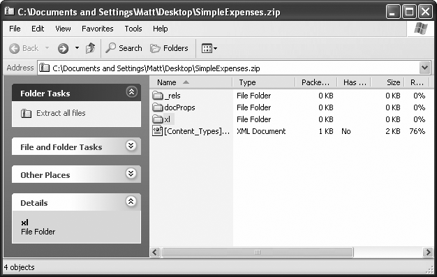
Figure 1-17. Inside every .xlsx file lurks a number of compressed files, each with different information. For example, separate files store printer settings, styles, the name of the person who created the document, the composition of your workbook, and each individual worksheet.
Tip
Don’t use the .xlsb format unless you’ve tried it out and find it really does give better performance for one of your spreadsheets. Usually, .xlsx and .xlsb are just as fast. And remember, the only time you’ll see any improvement is when you’re loading or saving a file. Once your spreadsheet is open in Excel, everything else (like scrolling around and performing calculations) happens at the same speed.
As you’ve just learned, Excel 2007 uses the same .xlsx file format as Excel 2010. That means that an Excel 2010 fan can exchange files with an Excel 2007 devotee, and there won’t be any technical problems.
However, there are still a few issues that can trip you up when sharing spreadsheets between Excel 2010 and Excel 2007. For example, Excel 2010 introduces a few new formula functions, such as RANK.AVG (LARGE(), SMALL(), and RANK(): Ranking Numbers). If you write a calculation that uses this function in Excel 2010, it won’t work when someone else opens the spreadsheet in Excel 2007. Instead of seeing the numeric result that you saw, they’ll see an error code mixed in with the rest of the spreadsheet data.
To avoid this sort of problem, you need the help of an Excel tool called the Compatibility Checker. The Compatibility Checker scans your spreadsheet to find features and formulas that will cause a problem in Excel 2007.
To use the Compatibility Checker, follow these steps:
Choose File→Info.
Excel switches into backstage view.
Click the Check for Issues button, and choose Check Compatibility.
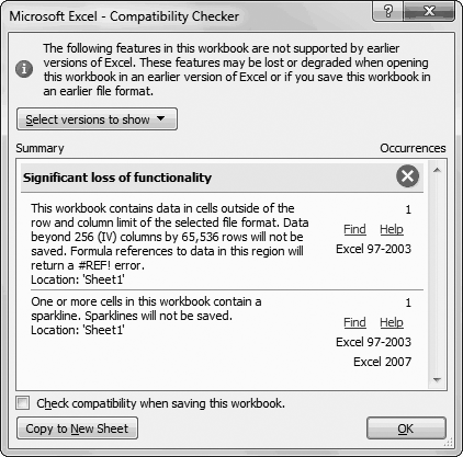
The Compatibility Checker scans your spreadsheet, looking for signs of trouble. It then reports any problems back to you (Figure 1-18).
Optionally, you can hide problems that don’t affect Excel 2007.
The Compatibility Checker reports on two types of problems. The first type of problems affect anyone who doesn’t have Excel 2010. These problems appear with the text “Excel 97-2003” and “Excel 2007” in the column on the right. The second problems affect Excel 2003 users but not Excel 2007 users. These problems appear with the text “Excel 97-2003” in the right column.
If you plan to share your spreadsheet file with Excel 2007 only, there’s no need to worry about Excel 2003 compatibility. You can hide these messages from the list by clicking the “Select versions to show” button and turning off Excel 97-2003.
You can choose to ignore the Compatibility Checker issues, click Find to hunt each one down, or click Help to figure out the exact problem. You can also click Copy to New Sheet to insert a full compatibility report into your spreadsheet as a separate worksheet. This way, you can print it up and review it in the comfort of your cubicle. (To get back to the worksheet with your data, click the Sheet1 tab at the bottom of the window. Chapter 4 has more about how to use and manage multiple worksheets.)
Note
The problems that the Compatibility Checker finds won’t cause serious errors, like crashing your computer or corrupting your data. That’s because Excel is designed to degrade gracefully. That means you can still open a spreadsheet that uses newer, unsupported features in an old version of Excel. However, you may receive a warning message and part of the spreadsheet may seem broken—that is, it won’t work as you intended.
Optionally, you can set the Compatibility Checker to run automatically for this workbook.
Turn on the “Check compatibility when saving this workbook” checkbox. Now, the Compatibility Checker will run each time you save your spreadsheet, just before the file is updated.
If you want to share your workbook with people who are using Excel 2003, the process is a bit more involved, because Excel 2003 uses the older .xls format instead of .xlsx.
When you find yourself in this situation, you have two choices:
Save your spreadsheet in the old format. You can save a copy of your spreadsheet in the traditional .xls Excel standard that’s been supported since Excel 97. To do so, choose File→Save As, and then, from the “Save as type” list, choose Excel 97-2003 Workbook.
Use a free add-in for older versions of Excel. People who are stuck with Excel 2000, Excel 2002, or Excel 2003 can read your Excel 2010 files—they just need a free add-in that’s provided by Microsoft. This is a good solution because it’s doesn’t require any work on your part. People with past-its-prime versions of Excel can find the add-in they need by surfing to www.microsoft.com/downloads and searching for “compatibility pack file formats” (or use the secret shortcut URL http://tinyurl.com/y5w78r). However, you should still run the Compatibility Checker to find out if your spreadsheet uses features that aren’t supported in Excel 2003.
Tip
When you save your Excel spreadsheet in another format, make sure to keep a copy in the standard .xlsx format. Why bother? Because other formats aren’t guaranteed to retain all your information, particularly if you choose a format that doesn’t support some of Excel’s newer features.
As you already know, each version of Excel introduces a small set of new features. Older versions of Excel don’t support these features. The differences between Excel 2007 and Excel 2010 are small. But the differences between Excel 2003 and Excel 2010 are more significant.
Excel tries to help you out in two ways. First, whenever you save a file in .xls format, Excel automatically runs the Compatibility Checker to review your spreadsheet and detect compatibility issues. Second, whenever you open a spreadsheet that’s in the old .xls file format, Excel switches into compatibility mode. While the Compatibility Checker points out potential problems after the fact, compatibility mode is designed to prevent you from using unsupported features in the first place. For example, in compatibility mode you’ll face these restrictions:
Excel limits you to a smaller grid of cells (65,536 rows instead of 1,048,576).
Excel prevents you from using really long or deeply nested formulas.
Excel doesn’t let you use some pivot table features.
In compatibility mode, these missing features aren’t anywhere to be found. In fact, compatibility mode is so seamless that you might not even notice you’re being limited. The only clear indication is the title bar at the top of the Excel window. Instead of seeing something like CateringList.xlsx, you’ll see CateringList.xls [Compatibility Mode].
Note
When you save an Excel workbook in .xls format, Excel won’t switch into compatibility mode right away. Instead, you need to close the workbook and reopen it.
If you decide at some point that you’re ready to move into the modern world and convert your file to the .xlsx format favored by Excel 2010, you can use the trusty File→Save As command. However, there’s an even quicker shortcut. Just choose File→Info, and click the Convert button. This saves an Excel 2010 version of your file with the same name but with the extension .xlsx, and reloads the file so you get out of compatibility mode. It’s up to you to delete your old .xls original if you don’t need it anymore.
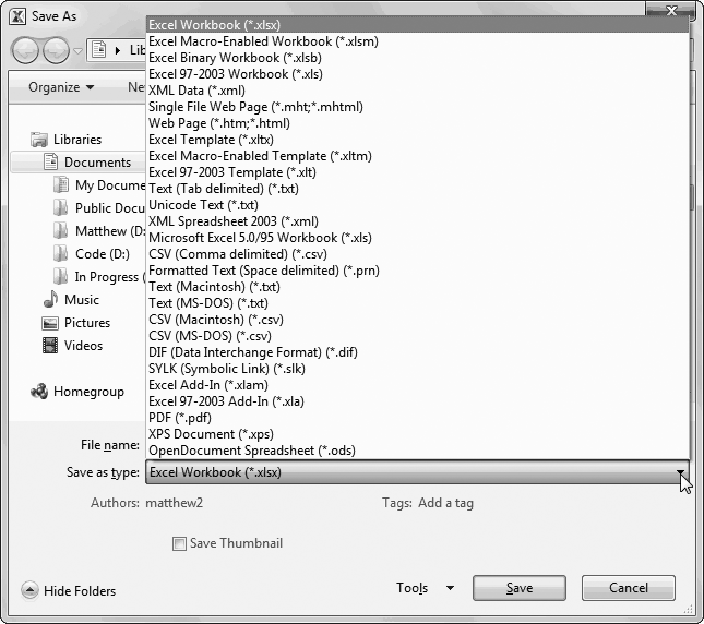
Some eccentric individuals have even older or stranger spreadsheet software on their computers. If you want to save a copy of your spreadsheet in a more exotic file type, you can choose File→Save As, and then find the desired format in the “Save as type” drop-down list (Figure 1-19). Alternatively, you can get quick access to the most popular file formats by choosing File→Save & Send and then clicking Change File Type. Double-click one of the file types that’s shown here to open the Save As dialog box with your choice already filled in the “Save as type” box.
Excel lets you save your spreadsheet using a variety of different formats, including the classic Excel 95 format from more than a decade ago. If you’re looking to view your spreadsheet using a mystery program, use the CSV file type, which produces a comma-delimited text file that almost all spreadsheet applications on any operating system can read (comma-delimited means the information has commas separating each cell).
Sometimes you want to save a copy of your spreadsheet so that people can read it even if they don’t have Excel (and even if they’re running a different operating system, like Linux or Apple’s OS X). In this situation, you have several choices:
Use the Excel Viewer. Even if you don’t have Excel, you can install a separate tool called the Excel Viewer, which is available from Microsoft’s website (search for “Excel Viewer” at http://www.microsoft.com/downloads). However, few people have the viewer, and even though it’s free, few want to bother installing it. And it doesn’t work on non-Windows computers.
Save your workbook as an HTML web page. That way, all you need to view the workbook is a web browser (and who doesn’t have one of those?). The only disadvantage is that you could lose complex formatting. Some worksheets may make the transition to HTML gracefully, while others don’t look very good when they’re squashed into a browser window. And if you’re planning to let other people print the exported worksheet, the results might be unsatisfactory. The next section has more about saving your worksheet as a web page.
Figure 1-19. Excel offers a few useful file type options in the “Save as type” list. CSV format is the best choice for compatibility with truly old software (or when nothing else seems to work). The four most commonly used formats—regular workbooks, macro-enabled workbooks, binary workbooks, and old-style Excel 2003 workbooks—sit at the top of the list.
Save your workbook as a PDF file. This gets you the best of both worlds—you keep all the rich formatting (so your workbook can be printed), and you let people who don’t have Excel (and possibly don’t even have Windows) view your work. Excel 2007 introduced the Save As PDF feature, but it forced Excel fans to download an add-in to get it. Excel 2010 has no such limitation. To save your spreadsheet as a PDF, you simply select File→Save As, and then pick PDF from the “Save as type” list. Or choose File→Save & Send, click Create PDF/XPS Document (in the “File Types” section), and then click the Create PDF/XPS button.
It doesn’t matter whether you use the File→Save As or the File→Save & Send approach. Either way, you end up at a modified version of the Save As dialog box that has a few additional options (Figure 1-20).
The “Publish as PDF” dialog box gives you some control over the quality settings with the “Optimize for” options. If you’re just saving a PDF copy so other people can view the information in your workbook, choose “Minimum size (publishing online)” to save some space. On the other hand, if there’s a possibility that the people reading your PDF might want to print it out, choose “Standard (publishing online and printing)” to save a slightly larger PDF that makes for a better printout.
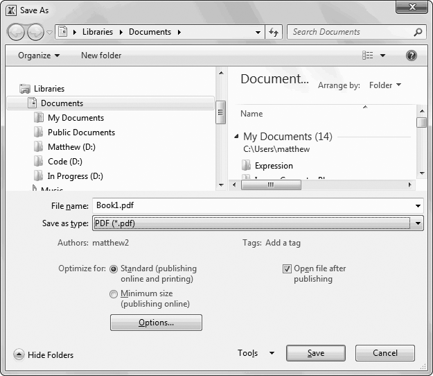
Figure 1-20. PDF files can be saved with different resolution and quality settings (which mostly affect any graphical objects like pictures and charts that you’ve placed in your workbook). Normally, you use higher quality settings if you’re planning to print your PDF file, because printers use higher resolutions than computer monitors.
You can switch on the “Open file after publishing” setting to tell Excel to open the PDF file in Adobe Reader (assuming you have it installed) after the publishing process is complete, so you can check the result.
Finally, if you want to publish only a portion of your spreadsheet as a PDF file, click the Options button to open a dialog box with even more settings. You can choose to publish just a fixed number of pages, just the selected cells, and so on. These options mirror the choices you get when sending a spreadsheet to the printer (How to Print an Excel File). You also see a few more cryptic options, most of which you can safely ignore. (They’re intended for PDF nerds.) One exception is the “Document properties” option—turn this off if you don’t want the PDF to keep track of certain information that identifies you, like your name. (Excel document properties are discussed in more detail on Document Properties.)
HTML (short for Hypertext Markup Language) is the language of the Web. Web authors use it to craft pages with text, links, and graphics.
In the early days of the Web, most programs had export-to-HTML features that weren’t worth a second glance. They distorted formatting, mangled text, and generated HTML so ugly that professional web developers fainted at the sight of it. Fortunately, the situation has improved. Though Excel’s HTML exporting might never match the graphical flair of the most talented web artists, it’s still downright impressive. Best of all, you can have your data ready for web surfers in a matter of minutes. Here’s what to do:
Choose File→Save As.
This action opens the Save As dialog box.
From the “Save as type” list, choose Web Page.
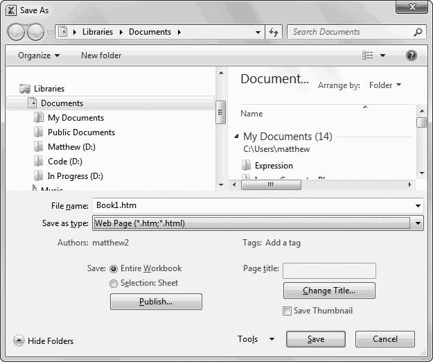
When you do, the Save As dialog box changes a little bit, as shown in Figure 1-21.
Choose which portion of your workbook you want to export to HTML.
If you want to export every worksheet, select Entire Workbook. If you just want to export the current worksheet, then select Selection: Sheet. (Every Excel workbook begins with three worksheets, and so far you’ve only used the first one. You’ll learn how to use the others—and add more—in Chapter 4.)
Tip
If you export the entire workbook, then Excel creates a web page that includes worksheet tab buttons, which you can use to switch from one worksheet to another. Generally, it’s simpler to just export a single worksheet—that makes more sense to web surfers.
Figure 1-21. When you’re saving a spreadsheet as a web page, the Save As dialog box gets a couple of new buttons. Use Change Title to set the web page’s title. You can also choose to save either the entire workbook or just the current selection.
If you select a group of cells before you choose File→Save, then you won’t see the Selection: Sheet option. Instead, you’ll see an option for the range of cells you chose, like “Selection: $A$2:$B$5.” (This means “the box of cells stretching from cell A2 in the top-left to cell B5 in the bottom-right.”) Choose this to create a web page that includes just that section of content.
If you want to add a title, click the Change Title button. When the Set Page Title dialog box appears, type in a title for your web page, and then click OK.
If you add a descriptive title, it appears in large bold font centered over the rest of your content. Titles don’t have any restrictions, so feel free to use something clear and descriptive like “Blue Skies Budget Report” or “Bankruptcy Projections for 2011.” This title also appears in the title bar of the web browser window. (Without the title information, most web browsers simply show the web page file name in their title bar.)
Browse to the location where you want to save the web page.
This location can be any of the places where you normally save files.
In the “File name” box, enter the name of the HTML file you want to create.
Depending on the content in your worksheet, Excel may create more than one file. If your worksheet contains embedded graphics or charts, or if you’re printing the entire workbook, Excel creates additional files. Excel puts these files in a newly created folder that has the same name as your file, plus the text “_files.”
If you save the web page BudgetReport.htm, Excel creates a folder named BudgetReport_files to hold the extra files. You need to keep the HTML file and this folder together at all times, because the folder contains some information that the HTML file uses. (The box on A Convenient Web Page Package has more about these folders.)
You now have a choice to either save or publish your web page.
If you want to perform a direct save of your file, effectively converting your current workbook into the HTML format, click the Save button. The original copy of your workbook remains in an .xlsx file, but Excel won’t update it again unless you choose File Menu→Save As and explicitly select it.
If you want to publish your file, which creates a copy of your data in the HTML format, click Publish. This launches the “Publish as Web Page” dialog box, which gives you a last-minute chance to select the portion of the workbook you want to publish and change the file name or web page title. You’ve already set all the options you need, so just click Publish to save your HTML file. Your workbook remains in the .xlsx format, but Excel makes an HTML copy suitable for viewing in your browser.
Note
When you use the “Publish as Web Page” dialog box, you can select “AutoRepublish every time this workbook is saved” to tell Excel to save the HTML copy of your workbook every time you save the .xlsx workbook file.
The exported copy of your worksheet is amazingly faithful. Excel preserves the formatting, layout, and content of your original worksheet. If your worksheet contains pictures or charts, Excel saves a separate graphic file for each object and displays it in the same web page using the linking power of HTML. Figure 1-22 shows an exported worksheet that includes a chart.
Note
It goes without saying that while other people can view an Excel-created web page, they can’t edit it. However, Excel 2010 blows the lid off this limitation with the Excel Web App—a simplified version of Excel that runs right in the browser. This tool is entirely free to use, even for people who don’t have the desktop version of Excel. Chapter 26 covers the Excel Web App in detail.
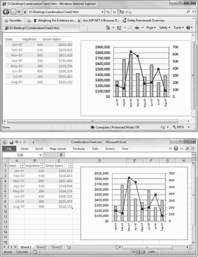
Figure 1-22. The HTML version of a spreadsheet, as displayed in Internet Explorer (top), mimics its appearance in Excel (bottom) with surprising accuracy. You need to get used to a few minor changes—like the fact that the HTML version doesn’t show any gridlines and can’t display nonstandard fonts. The solution? Stick to commonly supported Web fonts, like Arial, Courier New, Times New Roman, and Verdana (to name the most popular).
Occasionally, you might want to add confidential information to a spreadsheet—for example, a list of the airlines from which you’ve stolen spoons. If your computer is on a network, the solution may be as simple as storing your file in the correct, protected location. But if you’re afraid that you might inadvertently email the spreadsheet to the wrong people (say, executives at American Airlines), or if you’re about to expose systematic accounting irregularities in your company’s year-end statements, you’ll be happy to know that Excel provides a tighter degree of security. It allows you to password-protect your spreadsheets, which means anyone who wants to open them has to know the password you’ve set.
Excel actually has two layers of password protection that you can apply to a spreadsheet:
You can prevent others from opening your spreadsheet unless they know the correct password. This level of security, which scrambles your data for anyone without the password (a process known as encryption), is the strongest.
You can let others read a spreadsheet, but you can prevent them from modifying it unless they know the correct password.
You can apply one or both of these restrictions to a spreadsheet. Applying them is easy. Just follow these steps:
Choose File→Save As.
The Save As dialog box appears.
Click the Tools button, and then, from the pop-up menu, choose General Options.
If you’re using a Windows XP computer, you’ll find the Tools button in the bottom-left corner of the Save As dialog box. But if you’re running Windows Vista or Windows 7, it’s at the bottom right, just next to the Save button.
The General Options dialog box appears.
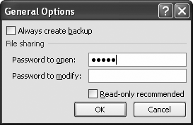
Type a password next to the security level you want to turn on (as shown in Figure 1-23). Then click OK.
The General Options dialog box also gives you a couple of other unrelated options:
Turn on the “Always create backup” checkbox if you want an extra copy of your file, just in case something goes wrong. (Think of it as insurance.) Excel creates a backup that has the file extension .xlk. For example, if you’re saving a workbook named SimpleExpenses.xlsx and you use the “Always create backup” option, Excel creates a file named “Backup of SimpleExpenses.xlk" every time you save your spreadsheet. You can open the .xlk file in Excel just like an ordinary Excel file. When you do, you see that it has an exact copy of your work.
Turn on the “Read-only recommended” checkbox to prevent other people from accidentally making changes to your spreadsheet. When you use this option, Excel shows a message every time you (or anyone else) opens the file. This message politely suggests that you open the spreadsheet in read-only mode, in which case Excel won’t allow any changes. Of course, it’s entirely up to the person opening the file whether to accept this recommendation.
Click Save to store the file.
If you use a password to restrict people from opening the spreadsheet, Excel prompts you to supply the “password to open” the next time you open the file (Figure 1-24, top).
If you use a password to restrict people from modifying the spreadsheet, the next time you open this file you’ll be given the choice—shown in Figure 1-24, bottom—to open it in read-only mode (which requires no password) or to open it in full edit mode (in which case you’ll need to supply the “password to modify”).
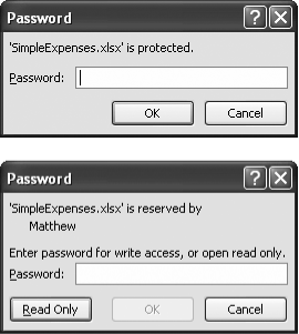
Figure 1-24. Top: You can give a spreadsheet two layers of protection. Assign a “password to open,” and you’ll see this window when you open the file Bottom: If you assign a “password to modify,” you’ll see the choices in this window. If you use both passwords, you’ll see both windows, one after the other.
The corollary to the edict “Save your data early and often” is the truism “Sometimes things fall apart quickly…before you’ve even had a chance to back up.” Fortunately, Excel includes an invaluable safety net called AutoRecover.
AutoRecover periodically saves backup copies of your spreadsheet while you work. If you suffer a system crash, you can retrieve the last AutoRecover backup even if you never managed to save the file yourself. Of course, even the AutoRecover backup won’t necessarily have all the information you entered in your spreadsheet before the problem occurred. But if AutoRecover saves a backup every 10 minutes (the standard), at most you’ll lose 10 minutes of work.
If your computer does crash, when you get it running again, you can easily retrieve your last AutoRecover backup. In fact, the next time you launch Excel, it automatically checks the backup folder and, if it finds a backup, it opens a Document Recovery panel on the left of the Excel window.
If your computer crashes mid-edit, the next time you open Excel you’ll probably see the same file listed twice in the Document Recovery window, as shown in Figure 1-25. The difference is the status. The status [AutoSaved] indicates the most recent backup created by Excel. The status [Original] indicates the last version of the file that you saved (which is safely stored on your hard drive, right where you expect it).
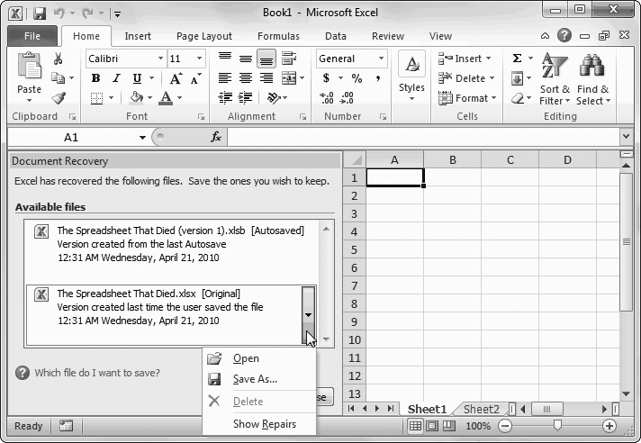
Figure 1-25. You can save or open an AutoRecover backup just as you would an ordinary Excel file; simply click the item in the list. Once you’ve dealt with all the backup files, close the Document Recovery window by clicking the Close button. If you haven’t saved your backup, Excel asks you at this point whether you want to save it permanently or delete the backup.
To open a file that’s in the Document Recovery window, just click it. You can also use a drop-down menu with additional options (Figure 1-24). Make sure to save the file before you leave Excel. After all, it’s just a temporary backup.
If you attempt to open a backup file that’s somehow been scrambled (technically known as corrupted), Excel automatically attempts to repair it. You can choose Show Repairs to display a list of any changes Excel had to make to recover the file.
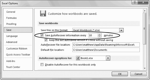
AutoRecover comes switched on when you install Excel, but you can tweak its settings. Choose File→Options, and then choose the Save section. Under the “Save workbooks” section, make sure that “Save AutoRecover information” is turned on.
You can also make a few other changes to AutoRecover settings:
You can adjust the backup frequency in minutes. (See Figure 1-26 for tips on timing.)
You can control whether Excel keeps a backup if you create a new spreadsheet, work on it for at least 10 minutes, and then close it without saving your work. This sort of AutoRecover backup is called a draft, and it’s discussed in more detail on AutoRecover. Ordinarily, the setting “Keep the last Auto Recovered file if I exit without saving” is switched on, and Excel keeps drafts. (To find all the drafts that Excel has saved for you, choose File→Recent and click the Recover Unsaved Workbooks link at the bottom of the window.)
Figure 1-26. You can configure how often AutoRecover saves backups. There’s really no danger in being too frequent. Unless you work with extremely complex or large spreadsheets—which might suck up a lot of computing power and take a long time to save—you can set Excel to save the document every five minutes with no appreciable slowdown.
You can choose the folder where you’d like Excel to save backup files. The standard folder works fine for most people, but feel free to pick some other place. Unfortunately, there’s no handy Browse button to help you find the folder, so you need to find the folder you want in advance (using a tool like Windows Explorer), write it down somewhere, and then copy the full folder path into this dialog box.
Under the “AutoRecover exceptions” heading, you can tell Excel not to bother saving a backup of a specific spreadsheet. Pick the spreadsheet name from the list (which shows all the currently open spreadsheet files), and then turn on the “Disable AutoRecover for this workbook only” setting. This setting is exceedingly uncommon, but you might use it if you have a gargantuan spreadsheet full of data that doesn’t need to be backed up. For example, this spreadsheet might hold records that you’ve pulled out of a central database so you can take a closer look. In this case, there’s no need to create a backup because your spreadsheet just has a copy of the data that’s in the database. (If you’re interested in learning more about this scenario, check out Chapter 23.)
Opening existing files in Excel works much the same as it does in any Windows program. To get to the standard Open dialog box, choose File→Open (or use the keyboard shortcut Ctrl+O). Using the Open dialog box, you can browse to find the spreadsheet file you want, and then click Open to load it into Excel.
Excel can open many file types other than its native .xlsx format. To learn the other formats it supports, launch the Open dialog box and, at the bottom, open the “Files of type” menu, which shows you the whole list. If you want to open a file but you don’t know what format it’s in, try using the first option on the menu, “All Files.” Once you choose a file, Excel scans the beginning of the file and informs you about the type of conversion it will attempt to perform (based on what type of file Excel thinks it is).
Note
Depending on your computer settings, Windows might hide file extensions. That means that instead of seeing the Excel spreadsheet file MyCoalMiningFortune.xlsx, you’ll just see the name MyCoalMiningFortune (without the .xlsx part on the end). In this case, you can still tell what the file type is by looking at the icon. If you see a small Excel icon next to the file name, that means Windows recognizes that the file is an Excel spreadsheet. If you see something else (like a tiny paint palette, for example), you need to make a logical guess about what type of file it is.
The Open dialog box also lets you open several spreadsheets in one step, as long as they’re all in the same folder. To use this trick, hold down the Ctrl key and click to select each file. Whe you click Open, Excel puts each one in a separate window, just as if you’d opened them one after the other.
Plan to take another crack at a recent spreadsheet? You can find the most recently opened documents in Excel’s Recent Documents list. To see this list, just choose File→Recent. The list holds 20 files. The best part about the Recent Documents list is the way you can pin a document there so it stays forever, as shown in Figure 1-27.
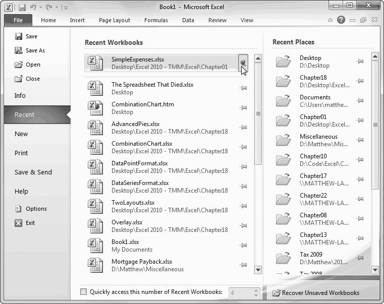
Figure 1-27. To keep a spreadsheet around on the Recent Documents list, click the thumbtack on the right. Excel moves your workbook to the top of the list and pins it in place. That means it won’t ever leave the list, no matter how many documents you open. If you decide to stop working with it later on, just click the thumbtack again to release it. Pinning is a great trick for keeping your most important files at your fingertips.
You can put recent documents even closer at hand by switching on the “Quickly access this number of Recent Workbooks” checkbox, which you’ll find underneath the list of recent documents. You can then enter a number in the adjacent box. For example, if you use 4 (the standard value), the four most recently used workbooks will appear directly in the column of commands on the left side of Excel’s backstage view. That means that if one of them is named MyFavoriteFile.xlsx, you can open it by choosing File→MyFavoriteFile.xlsx, rather than choosing File→Recent, and then clicking MyFavoriteFile.xlsx in the recent files list.
Tip
Do you want to hide your recent editing work? You can remove any file from the recent document list by right-clicking it and choosing “Remove from list.” And if the clutter is keeping you from finding the workbooks you want, just pin the important files, then right-click any file and choose “Clear unpinned workbooks.” This action removes every file that isn’t pinned down.
Just to the right of the Recent Documents list is the Recent Places list. It keeps track of the folders where you store your Excel files. So if you like to place Excel spreadsheets on your desktop and in your documents folder, you’ll see both folders in the list (as in in Figure 1-27). When you click a location, Excel heads to the appropriate location and shows the standard Open dialog box.
If you store your work in several different locations, far and wide, this feature can save you from digging through the directory tree. It’s particularly handy if you store documents on different drives or on a network. And just like the Recent Documents list, you can pin folders to the Recent Places list.
Even something that seems as innocent as an Excel file can’t always be trusted. Protected view is a new security feature in Excel 2010. It opens potentially risky Excel files in a specially limited Excel window. You’ll know that you’re in protected view because Excel doesn’t allow you to edit any of the data in the workbook, and it displays a message bar at the top of the window (Figure 1-28).
Excel automatically uses protected view when you download a spreadsheet from the Web or open it from your email inbox. This is actually a huge convenience, because Excel doesn’t need to hassle you with questions when you try to view the file (such as “are you sure you want to open this file?”). Because Excel’s protected view has bullet-proof security, it’s a safe way to view the most suspicious spreadsheet.
At this point, you’re probably wondering about the risks of rogue spreadsheets. Truthfully, they’re quite small. The most obvious danger is macro code: miniature programs that are stored in a spreadsheet file and can perform Excel tasks. Poorly written or malicious macro code can tamper with your Excel settings, lock up the program, and even scramble your data. But before you panic, consider this: Excel macro viruses are very rare, and the .xlsx file format doesn’t even allow macro code. Instead, macro-containing files must be saved as .xlsm or .xlsb files.
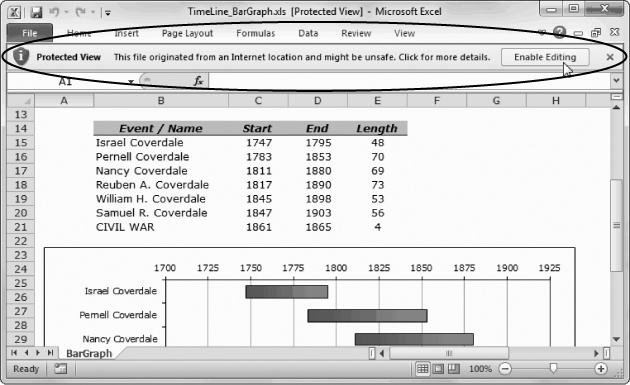
Figure 1-28. Currently, this file is in protected view. If you decide that it’s safe and you need to edit its content, click the Enable Editing button to open in the normal Excel window with no security safeguards.
The more subtle danger is that crafty hackers could create corrupted Excel files that might exploit tiny security holes in the program. One of these files could scramble Excel’s brains in a dangerous way, possibly causing it to execute a scrap of malicious computer code that could do almost anything. Once again, this sort of attack is extremely rare. It might not even be possible with the up-to-date .xlsx file format. But protected view completely removes any chance of an attack, which helps corporate bigwigs sleep at night.
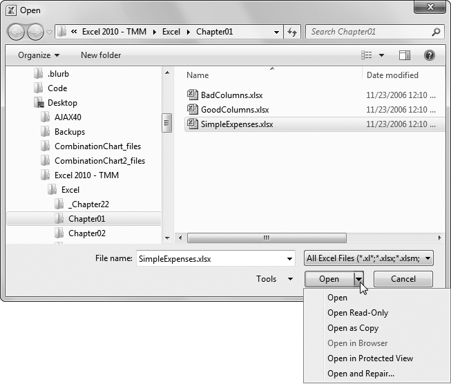
The Open dialog box harbors a few tricks. To see these hidden secrets, first select the file you want to use (by clicking it once, not twice), and then click the drop-down arrow on the right-side of the Open button. A menu with several additional options appears, as shown in Figure 1-29.
Here’s what these different choices do:
Open Read-Only opens the file, but won’t let you save changes. This option is great if you want to make sure you don’t accidentally overwrite an existing file. (For example, if you’re using last month’s sales invoice as a starting point for this month’s sales invoice, you might use Open Read-Only to make sure you can’t accidentally wipe out the existing file.) If you open a document in read-only mode, you can still make changes—you just have to save the file with a new file name (choose File→Save As).
Open as Copy creates a copy of the spreadsheet file in the same folder. If your file is named Book1.xlsx, the copy will be named “Copy of Book1.xlsx”. This feature comes in handy if you’re about to start editing a spreadsheet and want to be able to look at the last version you saved. Excel won’t let you open the same file twice. However, you can load the previous version by selecting the same file and using “Open as Copy”. (Of course, this technique works only when you have changes you haven’t saved yet. Once you save the current version of a file, the older version is overwritten and lost forever.)
Open in Browser is only available when you select an HTML file. This option allows you to open the HTML file in your computer’s web browser, which is something you’ll only want to attempt when trying to convert Excel files to web pages (Saving Your Spreadsheet As an HTML File).
Open in Protected View prevents a potentially dangerous file from running any code. However, you’ll also be restrained from editing the file, as explained on Protected View.
Open and Repair is useful if you need to open a file that’s corrupted. If you try to open a corrupted file by just clicking Open, Excel warns you that the file has problems and refuses to open it. To get around this problem, you can open the file using the “Open and Repair” option, which prompts Excel to make the necessary corrections, display them for you in a list, and then open the document. Depending on the type of problem, you might not lose any information at all.
As you open multiple spreadsheets, Excel creates a new window for each one. Although this helps keep your work separated, it can cause a bit of clutter and make it harder to track down the window you really want. Fortunately, Excel provides a couple of shortcuts that are indispensable when dealing with several spreadsheets at a time:
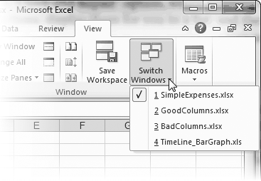
To jump from one spreadsheet to another, find the window in the View→Window→Switch Windows list, which includes the file name of all the currently open spreadsheets (Figure 1-30).
To move to the next spreadsheet, use the keyboard shortcut Ctrl+Tab or Ctrl+F6.
To move to the previous spreadsheet, use the shortcut key Ctrl+Shift+Tab or Ctrl+Shift+F6.
When you have multiple spreadsheets open at the same time, you need to take a little more care when closing a window so you don’t accidentally close the entire Excel application—unless you want to. Here are your choices:
You can close all the spreadsheets at once. To do so, you need to close the Excel window. Select File→Exit from any active spreadsheet, or just hold down Shift while you click the close icon (the infamous X button) in the top-right corner of the Excel window.
You can close a single spreadsheet. To do so, right-click the spreadsheet on the taskbar and click Close. Or switch to the spreadsheet you want to close (by clicking the matching taskbar button) and then choose File→Close.
Note
One of the weirdest limitations in Excel occurs if you try to open more than one file with the same name. No matter what steps you take, you can’t coax Excel to open both of them at once. It doesn’t matter if the files have different content or if they’re in different folders or even different drives. When you try to open a file that has the same name as a file that’s already open, Excel displays an error message and refuses to go any further. Sadly, the only solution is to open the files one at a time, or rename one of them.
Get Excel 2010: The Missing Manual now with the O’Reilly learning platform.
O’Reilly members experience books, live events, courses curated by job role, and more from O’Reilly and nearly 200 top publishers.

