Worksheets and Workbooks
Find and Replace
Spell Check
So Far, Youâve Learned How To Create A Basic Worksheet with a table of data. Thatâs great for getting started, but as power users, professional accountants, and other Excel jockeys quickly learn, some of the most compelling reasons to use Excel involve multiple tables that share information and interact with each other.
For example, say you want to track the performance of your company: you create one table summarizing your firmâs yearly sales, another listing expenses, and a third analyzing profitability and making predictions for the coming year. If you create these tables in different spreadsheet files, you have to copy shared information from one location to another, all without misplacing a number or making a mistake. And whatâs worse, with data scattered in multiple places, youâre missing the chance to use some of Excelâs niftiest charting and analytical tools. Similarly, if you try cramming a bunch of tables onto the same worksheet page, you can quickly create formatting and cell management problems.
Fortunately, a better solution exists. Excel lets you create spreadsheets with multiple pages of data, each of which can conveniently exchange information with other pages. Each page is called a worksheet, and a collection of one or more worksheets is called a workbook (which is also sometimes called a spreadsheet file). In this chapter, youâll learn how to manage the worksheets in a workbook. Youâll also take a look at two more all-purpose Excel features: Find and Replace (a tool for digging through worksheets in search of specific data) and the spell checker.
Many workbooks contain more than one table of information. For example, you might have a list of the items youâve purchased over two consecutive years. You might find it a bit challenging to arrange these different tables. You could stack them (Figure 4-1) or place them side by side (Figure 4-2), but neither solution is perfect.
Most Excel masters agree that the best way to arrange separate tables of information is to use separate worksheets for each table. When you create a new workbook, Excel automatically fills it with three blank worksheets named Sheet1, Sheet2, and Sheet3. Often, youâll work exclusively with the first worksheet (Sheet1), and not even realize that you have two more blank worksheets to play withânot to mention the ability to add plenty more.
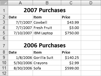
Figure 4-1. Stacking tables on top of each other is usually a bad idea. If you need to add more data to the first table, then you have to move the second table. Youâll also have trouble properly resizing or formatting columns because each column contains data from two different tables.
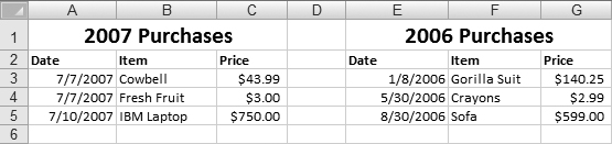
Figure 4-2. Youâre somewhat better off putting tables side by side, separated by a blank column, than you are stacking them, but this method can create problems if you need to add more columns to the first table. It also makes for a lot of side-to-side scrolling.
To move from one worksheet to another, you have a few choices:
Click the worksheet tabs at the bottom of Excelâs grid window (just above the status bar), as shown in Figure 4-3.
Press Ctrl+Page Down to move to the next worksheet. For example, if youâre currently in Sheet1, this key sequence jumps you to Sheet2.
Press Ctrl+Page Up to move to the previous worksheet. For example, if youâre currently in Sheet2, this key sequence takes you back to Sheet1.
Excel keeps track of the active cell in each worksheet. That means if youâre in cell B9 in Sheet1, and then move to Sheet2, when you jump back to Sheet1 youâll automatically return to cell B9.
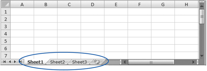
Figure 4-3. Worksheets provide a good way to organize multiple tables of data. To move from one worksheet to another, click the appropriate Worksheet tab at the bottom of the grid. Each worksheet contains a fresh grid of cells.
Tip
Excel includes some interesting viewing features that let you look at two different worksheets at the same time, even if these worksheets are in the same workbook. Youâll learn more about custom views in Chapter 6.
When you open a fresh workbook in Excel, you automatically get three blank worksheets in it. You can easily add more worksheets. Just click the Insert Worksheet button, which appears immediately to the right of your last worksheet tab (Figure 4-4). You can also use the Home â Cells â Insert â Insert Sheet command, which works the same way but inserts a new worksheet immediately to the left of the current worksheet. (Donât panic; Section 4.1.2 shows how you can rearrange worksheets after the fact.)
If you continue adding worksheets, youâll eventually find that all the worksheet tabs wonât fit at the bottom of your workbook window. If you run out of space, you need to use the scroll buttons (which are immediately to the left of the worksheet tabs) to scroll through the list of worksheets. Figure 4-5 shows the scroll buttons.
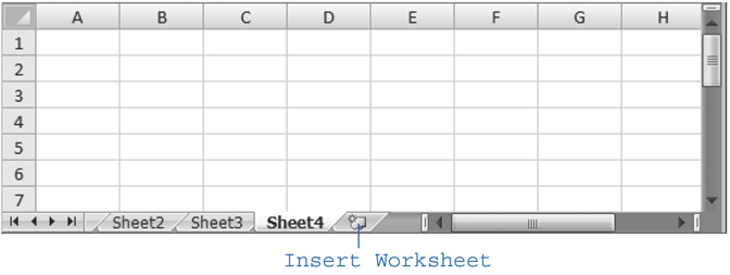
Figure 4-4. Every time you click the Insert Worksheet button, Excel inserts a new worksheet after your existing worksheets and assigns it a new name. For example, if you start with the standard Sheet1, Sheet2, and Sheet3 and click the Insert Worksheet button, then Excel adds a new worksheet namedâyou guessed itâSheet4.
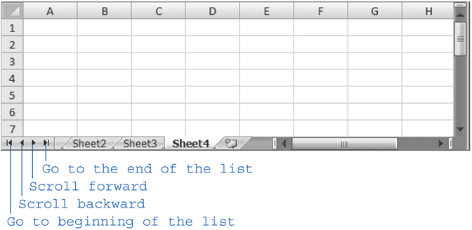
Figure 4-5. Using the scroll buttons, you can move between worksheets one at a time or jump straight to the first or last tab. These scroll buttons control only which tabs you seeâyou still need to click the appropriate tab to move to the worksheet you want to work on.
Tip
If you have a huge number of worksheets and they donât all fit in the strip of worksheet tabs, thereâs an easier way to jump around. Right-click the scroll buttons to pop up a list with all your worksheets. You can then move to the worksheet you want by clicking it in the list.
Removing a worksheet is just as easy as adding one. Simply move to the worksheet you want to get rid of, and then choose Home â Cells â Delete â Delete Sheet (you can also right-click a worksheet tab and choose Delete). Excel wonât complain if you ask it to remove a blank worksheet, but if you try to remove a sheet that contains any data, it presents a warning message asking for your confirmation. Also, if youâre down to one last worksheet, Excel wonât let you remove it. Doing so would create a tough existential dilemma for Excelâa workbook that holds no work-sheetsâso the program prevents you from taking this step.
Warning
Be careful when deleting worksheets, as you canât use Undo (Ctrl+Z) to reverse this change! Undo also doesnât work to reverse a newly inserted sheet.
Excel starts you off with three worksheets for each workbook, but changing this settingâs easy. You can configure Excel to start with fewer worksheets (as few as one), or many more (up to 255). Select Office button â Excel Options, and then choose the Popular section. Under the heading âWhen creating new workbooksâ change the number in the âInclude this many sheetsâ box, and then click OK. This setting takes effect the next time you create a new workbook.
Note
Although youâre limited to 255 sheets in a new workbook, Excel doesnât limit how many worksheets you can add after youâve created a workbook. The only factor that ultimately limits the number of worksheets your workbook can hold is your computerâs memory. However, modern day PCs can easily handle even the most ridiculously large, worksheet stuffed workbook.
Deleting worksheets isnât the only way to tidy up a workbook or get rid of information you donât want. You can also choose to hide a worksheet temporarily. When you hide a worksheet, its tab disappears but the worksheet itself remains part of your spreadsheet file, available whenever you choose to unhide it. Hidden worksheets also donât appear on printouts. To hide a worksheet, right-click the worksheet tab and choose Hide. (Or, for a more long-winded approach, choose Home â Cells â Format â Hide & Unhide â Hide Sheet.)
To redisplay a hidden worksheet, right-click any worksheet tab and choose Unhide. The Unhide dialog box appears along with a list of all hidden sheets, as shown in Figure 4-6. You can then select a sheet from the list and click OK to unhide it. (Once again, the ribbon can get you the same windowâjust point yourself to Home â Cells â Format â Hide & Unhide â Unhide Sheet.)
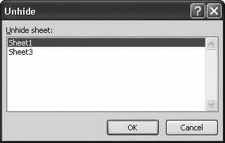
Figure 4-6. This workbook contains two hidden worksheets. To restore one, just select it from the list, and then click OK. Unfortunately, if you want to show multiple hidden sheets, you have to use the Unhide Sheet command multiple times. Excel has no shortcut for unhiding multiple sheets at once.
The standard names Excel assigns to new worksheetsâSheet1, Sheet2, Sheet3, and so onâarenât very helpful for identifying what they contain. And they become even less helpful if you start adding new worksheets, since the new sheet numbers donât necessarily indicate the position of the sheets, just the order in which you created them.
For example, if youâre on Sheet 3 and you add a new worksheet (by choosing Home â Cells â Insert â Insert Sheet), then the worksheet tabs read: Sheet1, Sheet2, Sheet4, Sheet3. (Thatâs because the Insert Sheet command inserts the new sheet just before your current sheet.) Excel doesnât expect you to stick with these auto-generated names. Instead, you can rename them by right-clicking the worksheet tab and selecting Rename, or just double-click the sheet name. Either way, Excel highlights the worksheet tab, and you can type a new name directly onto the tab. Figure 4-7 shows worksheet tabs with better names.
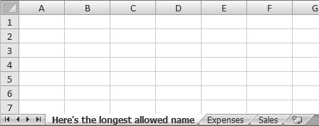
Figure 4-7. Worksheet names can be up to 31 characters long and can include letters, numbers, some symbols, and spaces.
Note
Excel has a small set of reserved names that you can never use. To witness this problem, try to create a worksheet named History. Excel doesnât let you because it uses the History worksheet as part of its change tracking features. Use this Excel oddity to impress your friends.
Sometimes Excel refuses to insert new worksheets exactly where youâd like them. Fortunately, you can easily rearrange any of your worksheets just by dragging their tabs from one place to another, as shown in Figure 4-8.
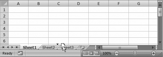
Figure 4-8. When you drag a worksheet tab, a tiny page appears beneath the arrow cursor. As you move the cursor around, youâll see a black triangle appear, indicating where the worksheet will land when you release the mouse button.
Tip
You can use a similar technique to create copies of a worksheet. Click the worksheet tab and begin dragging, just as you would to move the worksheet. However, before releasing the mouse button, press the Ctrl key (youâll see a plus sign [+] appear). When you let go, Excel creates a copy of the worksheet in the new location. The original worksheet remains in its original location. Excel gives the new worksheet a name with a number in parentheses. For example, a copy of Sheet1 is named Sheet1 (2). As with any other worksheet tab, you can change this name.
When youâre dealing with great mounds of information, you may have a tough time ferreting out the nuggets of data you need. Fortunately, Excelâs find feature is great for helping you locate numbers or text, even when theyâre buried within massive workbooks holding dozens of worksheets. And if you need to make changes to a bunch of identical items, the find-and-replace option can be a real timesaver.
The âFind and Replaceâ feature includes both simple and advanced options. In its basic version, youâre only a quick keystroke combo away from a word or number you know is lurking somewhere in your data pile. With the advanced options turned on, you can do things like search for cells that have certain formatting characteristics and apply changes automatically. The next few sections dissect these features.
Excelâs find feature is a little like the Go To tool described in Chapter 1, which lets you move across a large expanse of cells in a single bound. The difference is that Go To moves to a known location, using the cell address you specify. The find feature, on the other hand, searches every cell until it finds the content youâve asked Excel to look for. Excelâs search works similarly to the search feature in Microsoft Word, but itâs worth keeping in mind a few additional details:
Excel searches by comparing the content you enter with the content in each cell. For example, if you searched for the word Date, Excel identifies as a match a cell containing the phrase Date Purchased.
When searching cells that contain numeric or date information, Excel always searches the display text. For example, say a cell displays dates using the day-month-year format, like 2-Dec-05. You can find this particular cell by searching for any part of the displayed date (using search strings like Dec or 2-Dec-05). But if you use the search string 12/2/2005, you wonât find a match because the search string and the display text are different. A similar behavior occurs with numbers. For example, the search strings $3 and 3.00 match the currency value $3.00. However, the search string 3.000 wonât turn up anything because Excel wonât be able to make a full text match.
Excel searches one cell at a time, from left to right. When it reaches the end of a row, it moves to the first column of the next row.
To perform a find operation, follow these steps:
Move to the cell where you want the search to begin.
If you start off halfway down the worksheet, for example, the search covers the cells from there to the end of the worksheet, and then âloops overâ and starts at cell A1. If you select a group of cells, Excel restricts the search to just those cells. You can search across a set of columns, rows, or even a non-contiguous group of cells.
Choose Home â Editing â Find & Select â Find, or press Ctrl+F.
The "Find and Replaceâ window appears, with the Find tab selected.
Note
To assist frequent searches, Excel lets you keep the "Find and Replaceâ window hanging around (rather than forcing you to use it or close it, as is the case with many other dialog boxes). You can continue to move from cell to cell and edit your worksheet data even while the "Find and Replaceâ window remains visible.
In the âFind whatâ combo box, enter the word, phrase, or number youâre looking for.
If youâve performed other searches recently, you can reuse these search terms. Just choose the appropriate search text from the âFind whatâ drop-down list.
Click Find Next.
Excel jumps to the next matching cell, which becomes the active cell. However, Excel doesnât highlight the matched text or in any way indicate why it decided the cell was a match. (Thatâs a bummer if youâve got, say, 200 words crammed into a cell.) If it doesnât find a matching cell, Excel displays a message box telling you it couldnât find the requested content.
If the first match isnât what youâre looking for, you can keep looking by clicking Find Next again to move to the next match. Keep clicking Find Next to move through the worksheet. When you reach the end, Excel resumes the search at the beginning of your worksheet, potentially bringing you back to a match youâve already seen. When youâre finished with the search, click Close to get rid of the âFind and Replaceâ window.
One of the problems with searching in Excel is that youâre never quite sure how many matches there are in a worksheet. Sure, clicking Find Next gets you from one cell to the next, but wouldnât it be easier for Excel to let you know right away how many matches it found?
Enter the Find All feature. With Find All, Excel searches the entire worksheet in one go, and compiles a list of matches, as shown in Figure 4-9.
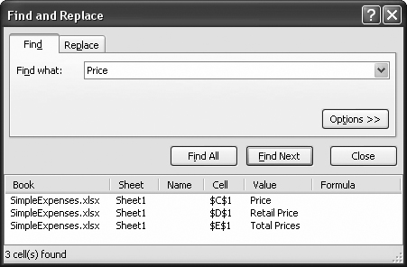
Figure 4-9. In the example shown here, the search for Price matched three cells in the worksheet. The list shows you the complete text in the matching cell and the cell reference (for example, $C$1, which is a reference to cell C1).
The Find All button doesnât lead you through the worksheet like the find feature. Itâs up to you to select one of the results in the list, at which point Excel automatically moves you to the matching cell.
The Find All list wonât automatically refresh itself: After youâve run a Find All search, if you add new data to your worksheet, you need to run a new search to find any newly added terms. However, Excel does keep the text and numbers in your found-items list synchronized with any changes you make in the worksheet. For example, if you change cell D5 to Total Price, the change appears in the Value column in the found-items list automatically. This tool is great for editing a worksheet because you can keep track of multiple changes at a single glance.
Finally, the Find All feature is the heart of another great Excel guru trick: it gives you another way to change multiple cells at once. After youâve performed the Find All search, select all the entries you want to change from the list by clicking them while you hold down Ctrl (this trick allows you to select several at once). Click in the formula bar, and then start typing the new value. When youâre finished, hit Ctrl+Enter to apply your changes to every selected cell. Voilà âitâs like "Find and Replaceâ, but youâre in control!
Basic searches are fine if all you need to find is a glaringly unique phrase or number (Pet Snail Names or 10,987,654,321). But Excelâs advanced search feature gives you lots of ways to fine-tune your searches or even search more than one worksheet. To conduct an advanced search, begin by clicking the "Find and Replaceâ windowâs Options button, as shown in Figure 4-10.
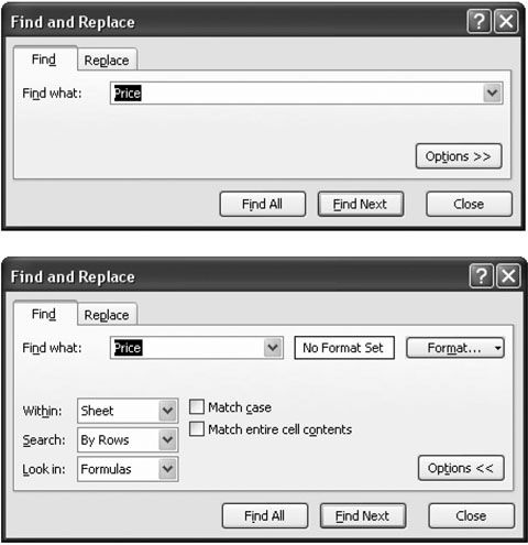
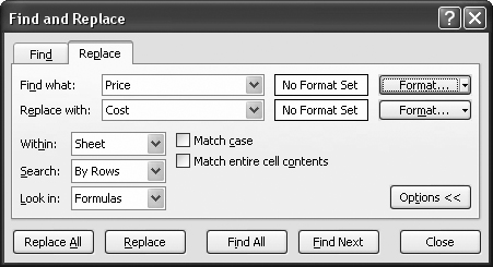
Figure 4-10. In the standard âFind and Replaceâ window (top), when you click Options, Excel gives you a slew of additional settings (bottom) so you can configure things like search direction, case sensitivity, and format matching.
You can set any or all of the following options:
If you want your search to span multiple worksheets, go to the Within box, and then choose Workbook. The standard option, Sheet, searches all the cells in the currently active worksheet. If you want to continue the search in the other worksheets in your workbook, choose Workbook. Excel examines the worksheets from left to right. When it finishes searching the last worksheet, it loops back and starts examining the first worksheet.
The Search pop-up menu lets you choose the direction you want to search. The standard option, By Rows, completely searches each row before moving on to the next one. That means that if you start in cell B2, Excel searches C2, D2, E2, and so on. Once itâs moved through every column in the second row, it moves onto the third row and searches from left to right.
On the other hand, if you choose By Columns, Excel searches all the rows in the current column before moving to the next column. That means that if you start in cell B2, Excel searches B3, B4, and so on until it reaches the bottom of the column and then starts at the top of the next column (column C).
The "Match caseâ option lets you specify whether capitalization is important. If you select âMatch caseâ, Excel finds only words or phrases whose capitalization matches. Thus, searching for Date matches the cell value Date, but not date.
The âMatch entire cell contentsâ option lets you restrict your searches to the entire contents of a cell. Excel ordinarily looks to see if your search term is contained anywhere inside a cell. So, if you specify the word Price, Excel finds cells containing text like Current Price and even Repriced Items. Similarly, numbers like 32 match cell values like 3253, 10032, and 1.321. Turning on the âMatch entire cell contentsâ option forces Excel to be precise.
Note
Remember, Excel searches for numbers as theyâre displayed (as opposed to looking at the underlying values that Excel uses to store numbers internally). That means that if youâre searching for a number formatted using the dollar Currency format ($32.00, for example), and youâve turned on the âMatch entire cell contentsâ checkbox, youâll need to enter the number exactly as it appears on the worksheet. Thus, $32.00 would work, but 32 alone wonât help you.
Excelâs "Find and Replaceâ is an equal opportunity search tool: It doesnât care what the contents of a cell look like. But what if you know, for example, that the data youâre looking for is formatted in bold, or that itâs a number that uses the Currency format? You can use these formatting details to help Excel find the data you want and ignore cells that arenât relevant.
To use formatting details as part of your search criteria, follow these steps:
Launch the Find tool.
Choose Home â Editing â Find & Select â Find, or press Ctrl+F. Make sure that the âFind and Replaceâ window is showing the advanced options (by clicking the Options button).
Click the Format button next to the "Find whatâ search box.
The Find Format dialog box appears (Figure 4-11). It contains the same options as the Format Cell dialog box discussed in Section 5.1.
Figure 4-11. In the Find Format dialog box, Excel wonât use any formatting option thatâs blank or grayed out as part of itâs search criteria. For example, here, Excel wonât search based on alignment. Checkboxes are a little trickier. In some versions of Windows, it looks like the checkbox is filled with a solid square (as with the âMerge cellsâ setting in this example). In other versions of Windows, it looks like the checkbox is dimmed and checked at the same time. Either way, this visual cue indicates that Excel wonât use the setting as part of its search.
Specify the format settings you want to look for.
Using the Find Format dialog box, you can specify any combination of number format, alignment, font, fill pattern, borders, and formatting. Chapter 5 explains all these formatting settings in detail.
When youâre finished, click OK to return to the "Find and Replaceâ window.
Next to the âFind whatâ search box, a preview appears indicating the formatting of the cell that youâll be searching for, as shown in Figure 4-12.
To remove these formatting restrictions, click the pop-up menu to the right of the Format button and then choose Clear Find.
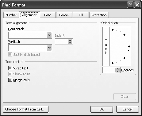
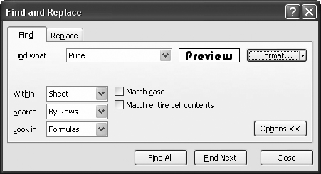
Figure 4-12. The Find Format dialog box shows a basic preview of your formatting choices. In this example, the search will find cells containing the word Price that also use white lettering, a black background, and the Bauhaus font.
Tip
Rather than specifying all the format settings manually, you can copy them from another cell. Just click the Choose Format From Cell button at the bottom of the Find Format dialog box. The pointer changes to a plus symbol with an eyedropper next to it. Next, click any cell that has the formatting you want to match. Keep in mind that when you use this approach, you copy all the format settings.
You can use Excelâs search muscles to find not only the information youâre interested in, but also to modify cells quickly and easily. Excel lets you make two types of changes using its replace tool:
You can automatically change cell content. For example, you can replace the word Colour with Color or the number $400 with $40.
You can automatically change cell formatting. For example, you can search for every cell that contains the word Price or the number $400 and change the fill color. Or, you can search for every cell that uses a specific font, and modify these cells so they use a new font.
Hereâs how to perform a replace operation. The box below gives some super-handy tricks you can do with this process.
Move to the cell where the search should begin.
Remember, if you donât want to search the entire spreadsheet, just select the range of cells you want to search.
Choose Home â Editing â Find & Select â Replace, or press Ctrl+H.
The "Find and Replaceâ window appears, with the Replace tab selected, as shown in Figure 4-13.
In the âFind whatâ box, enter your search term. In the âReplace withâ box, enter the replacement text.
Type the replacement text exactly as you want it to appear. If you want to set any advanced options, click the Options button (see the earlier sections âMore Advanced Searchesâ and âFinding Formatted Cellsâ for more on your choices).
Perform the search.
Youâve got four different options here. Replace All immediately changes all the matches your search identifies. Replace changes only the first matched item (you can then click Replace again to move on to subsequent matches or to select any of the other three options). Find All works just like the same feature described in the box in Section 4.2.5. Find Next moves to the next match, where you can click Replace to apply your specified change, or click any of the other three buttons. The replace options are good if youâre confident you want to make a change; the find options work well if you first want to see what changes youâre about to make (although you can reverse either option using Ctrl+Z to fire off the Undo command).
A spell checker in Excel? Is that supposed to be for people who canât spell 138 correctly? The fact is that more and more people are cramming textâcolumn headers, boxes of commentary, lists of favorite cereal combinationsâinto their spreadsheets. And Excelâs designers have graciously responded by providing the very same spell checker that youâve probably used with Microsoft Word. As you might expect, Excelâs spell checker examines only text as it sniffs its way through a spreadsheet.
Note
The same spell checker works in almost every Office application, including Word, PowerPoint, and Outlook.
To start the spell checker, follow these simple steps:
Move to where you want to start the spell check.
If you want to check the entire worksheet from start to finish, move to the first cell. Otherwise, move to the location where you want to start checking. Or, if you want to check a portion of the worksheet, select the cells you want to check.
Unlike the âFind and Replaceâ feature, Excelâs spell check can check only one worksheet at a time.
Choose Review â Proofing â Spelling, or press F7.
The Excel spell checker starts working immediately, starting with the current cell and moving to the right, going from column to column. After it finishes the last column of the current row, checking continues with the first column of the next row.
If you donât start at the first cell (A1) in your worksheet, Excel asks you when it reaches the end of the worksheet whether it should continue checking from the beginning of the sheet. If you say yes, it checks the remaining cells and stops when it reaches your starting point (having made a complete pass through all of your cells).
When the spell check finishes, a dialog box informs you that all cells have been checked. If your cells pass the spell check, this dialog box is the only feedback you receive. On the other hand, if Excel discovers any potential spelling errors during its check, it displays a Spelling window, as shown in Figure 4-14, showing the offending word and a list of suggestions.
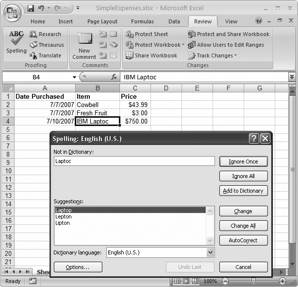
Figure 4-14. When Excel encounters a word it thinks is misspelled, it displays the Spelling window. The cell containing the wordâbut not the actual word itselfâgets highlighted with a black border. Excel doesnât let you edit your file while the Spelling window is active. You either have to click one of the options on the Spelling window or cancel the spell check.
The Spelling window offers a wide range of choices. If you want to use the list of suggestions to perform a correction, you have three options:
Click one of the words in the list of suggestions, and then click Change to replace your text with the proper spelling. Double-clicking the word has the same effect.
Click one of the words in the list of suggestions, and click Change All to replace your text with the proper spelling. If Excel finds the same mistake elsewhere in your worksheet, it repeats the change automatically.
Click one of the words in the list of suggestions, and click AutoCorrect. Excel makes the change for this cell, and for any other similarly misspelled words. In addition, Excel adds the correction to its AutoCorrect list (described in Section 2.2.2). That means if you type the same unrecognized word into another cell (or even another workbook), Excel automatically corrects your entry. This option is useful if youâve discovered a mistake that you frequently make.
Tip
If Excel spots an error but it doesnât give you the correct spelling in its list of suggestions, just type the correction into the âNot in Dictionaryâ box and hit Enter. Excel inserts your correction into the corresponding cell.
On the other hand, if Excel is warning you about a word that doesnât represent a mistake (like your company name or some specialized term), you can click one of the following buttons:
Ignore Once skips the word and continues the spell check. If the same word appears elsewhere in your spreadsheet, Excel prompts you again to make a correction.
Ignore All skips the current word and all other instances of that word throughout your spreadsheet. You might use Ignore All to force Excel to disregard something you donât want to correct, like a personâs name. The nice thing about Ignore All is that Excel doesnât prompt you again if it finds the same name, but it does prompt you again if it finds a different spelling (for example, if you misspelled the name).
Add to Dictionary adds the word to Excelâs custom dictionary. Adding a word is great if you plan to keep using a word thatâs not in Excelâs dictionary. (For example, a company name makes a good addition to the custom dictionary.) Not only does Excel ignore any occurrences of this word, but if it finds a similar but slightly different variation of that word, it provides the custom word in its list of suggestions. Even better, Excel uses the custom dictionary in every workbook you spell check.
Cancel stops the operation altogether. You can then correct the cell manually (or do nothing) and resume the spell check later.
Excel lets you tweak how the spell checker works by letting you change a few basic options that control things like the language used and which, if any, custom dictionaries Excel examines. To set these options (or just to take a look at them), choose Office button â Excel Options, and then select the Proofing section (Figure 4-15). You can also reach these options by clicking the Spelling windowâs Options button while a spell check is underway.
The most important spell check setting is the language (at the bottom of the window), which determines what dictionary Excel uses. Depending on the version of Excel that youâre using and the choices you made while installing the software, you might be using one or more languages during a spell check operation.
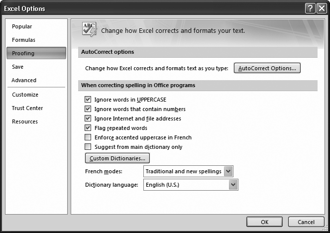
Figure 4-15. The spell checker options allow you to specify the language and a few other miscellaneous settings. This figure shows the standard settings that Excel uses when you first install it.
Some of the other spelling options you can set include:
Ignore words in UPPERCASE. If you choose this option, Excel wonât bother checking any word written in all capitals (which is helpful when your text contains lots of acronyms).
Ignore words that contain numbers. If you choose this option, Excel wonât check words that contain numeric characters, like Sales43 or H3ll0. If you donât choose this option, Excel flags these entries as errors unless youâve specifically added them to the custom dictionary.
Ignore Internet and file addresses. If you choose this option, Excel ignores words that appear to be file paths (like C:\Documents and Settings) or Web site addresses (like http://FreeSweatSocks.com).
Flag repeated words. If you choose this option, Excel treats words that appear consecutively (âthe theâ) as an error.
Suggest from main dictionary only. If you choose this option, the spell checker doesnât suggest words from the custom dictionary. However, it still accepts a word that matches one of the custom dictionary entries.
You can also choose the file Excel uses to store custom wordsâthe unrecognized words that you add to the dictionary while a spell check is underway. Excel automatically creates a file named custom.dic for you to use, but you might want to use another file if youâre sharing someone elseâs custom dictionary. (You can use more than one custom dictionary at a time. If you do, Excel combines them all to get one list of custom words.) Or, you might want to edit the list of words if youâve mistakenly added something that shouldnât be there.
To perform any of these tasks, click the Custom Dictionaries button, which opens the Custom Dictionaries dialog box (Figure 4-16). From this dialog box, you can remove your custom dictionary, change it, or add a new one.
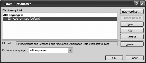
Figure 4-16. Excel starts you off with a custom dictionary named custom.dic (shown here). To add an existing custom dictionary, click Add and browse to the file. Or, click New to create a new, blank custom dictionary. You can also edit the list of words a dictionary contains (select it and click Edit Word List). Figure 4-17 shows an example of dictionary editing.
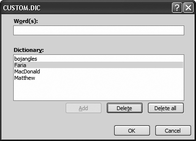
Figure 4-17. This custom dictionary is fairly modest. It contains three names and an unusual word. Excel lists the words in alphabetical order. You can add a new word directly from this window (type in the text and click Add), remove one (select it and click Delete), or go nuclear and remove them all (click Delete All).
Note
All custom dictionaries are ordinary text files with the extension .dic. Unless you tell it otherwise, Excel assumes that custom dictionaries are located in the Application Data\Microsoft\UProof folder in the folder Windows uses for user-specific settings. For example, if youâre logged in under the user account Brad_Pitt, youâd find the custom dictionary in the C:\Documents and Settings\Brad_Pitt\Application Data\ Microsoft\ UProof folder.
Get Excel 2007 for Starters: The Missing Manual now with the O’Reilly learning platform.
O’Reilly members experience books, live events, courses curated by job role, and more from O’Reilly and nearly 200 top publishers.

