Discrete Stochastic Processes and Optimal Filtering

2.4. Affine transformation of a Gaussian vector

We can generalize to vectors the following result on Gaussian r.v.:

If Y ∼ N (m, σ²) then ∀a, b ∈ aY + b ∼ N (am + b, a² σ²).

By modifying a little the annotation, with N (am + b, a² σ²) becoming N (am + b, a VarYa), we can imagine already how this result is going to extend to Gaussian vectors.

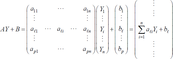
PROPOSITION.– Given a Gaussian vector Y ∼ N_n (m, Γ_Y), A a matrix belonging to M (p, n) and a certain vector B ∈ ^p, then AY + B is a Gaussian vector ∼ N_p (Am + B, AΓ_Y A^T).

DEMONSTRATION.–

– this is indeed a Gaussian vector (of dimension p) because every linear combination of its components is an affine combination of the r.v. Y₁,…, Y_i,…, Y_n and by hypothesis Y^T = (Y₁,…, Y_n) is a Gaussian vector;

– furthermore, we have seen that if Y is a 2^nd order vector:

E(AY + B) = AEY + B = Am + B and Γ_AY+B = AΓ_YA^T.

EXAMPLE.– Given (n + 1) independent r.v. Y_j ∼ N (μ, σ²) j = 0 at n, it emerges Y^T = (Y₀, Y₁,…, Y_n) ∼ N_n+1 (m, Γ_Y) with m^T = (μ,…, μ) and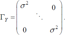

Furthermore, given new r.v. X defined by:

X₁ = Y₀ + Y₁,…, X_n = Y_n−1 + Y_n,

the vector X^T = (X_l,…, X_n) is Gaussian ...