Discrete Stochastic Processes and Optimal Filtering

2.1. Some reminders regarding random Gaussian vectors

DEFINITION.– We say that a real r.v. is Gaussian, of expectation m and of variance σ² if its law of probability P_X :

– admits the density 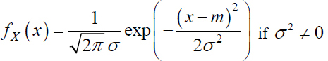(using a double integral calculation, for example, we can verify that f_X (x)dx = 1);

– is the Dirac measure δ_m if σ² = 0.

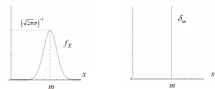
Figure 2.1. Gaussian density and Dirac measure

If σ² ≠ 0, we say that X is a non-degenerate Gaussian r.v.

If σ² = 0, we say that X is a degenerate Gaussian r.v.; X is in this case a “certain r.v.” taking the value m with the probability 1.

EX = m, Var X = σ². This can be verified easily by using the probability distribution function.

As we have already observed, in order to specify that an r.v. X is Gaussian of m expectation and of σ² variance, we will write X ∼ N (m, σ²).

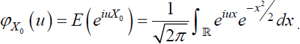
Characteristic function of X ∼ N (m, σ²)

Let us begin firstly by determining the characteristic function of X₀ ~ N (0, 1):

We can easily see that the theorem of derivation under the sum sign can be applied:

Following this by integration by parts:

The resolution of the differential equation with the condition ...