Digital Signal Processing Using Matlab

14.2. Solved exercises

EXERCISE 14.1.

Perform the DCT compression of the image “dots”, which can be found in the file “imdemos” of the image processing toolbox. Use the MATLAB function dct2.m

a. Plot the mean square error variation with the number of conserved coefficients.

b. Perform the image compression by preserving only the 1,024 largest coefficients.

a.

load imdemos dots;
[N1,N2]=size(dots);
sl=double(dots); s=zeros(N1,N2);
s=sl; y=dct2(s); [ly,cy]=size(y);
yv=y(:); [yvs,idxs]=sort(abs(yv));
yvs=flipud(yvs); idxs=flipud(idxs);
cont=0;
for r=2.^[0 :14]
    yvr=yv ; yr=y;
    yvr(idxs(r+1 :N1*N2))=zeros(N1*N2-r,1);
    for k=1:N2
        yr(:,k)=yvr((k-1)*N1+1:k*N1,1);

end
  sr=idct2(yr); cont=cont+1;
  eqm(cont)=(sum(sum(s-sr).^2))/(N1*N2);
end
plot(eqm);
set(gca,'XTickLabel',2.^(str2num(get(gca,'XTickLabel'))-1))
xlabel('Number of preserved coefficients');
ylabel('Error'); title('Variation of the mean square error')

Note that the mean square error decreases very fast with the number of conserved coefficients due to the high redundancy of the original image.

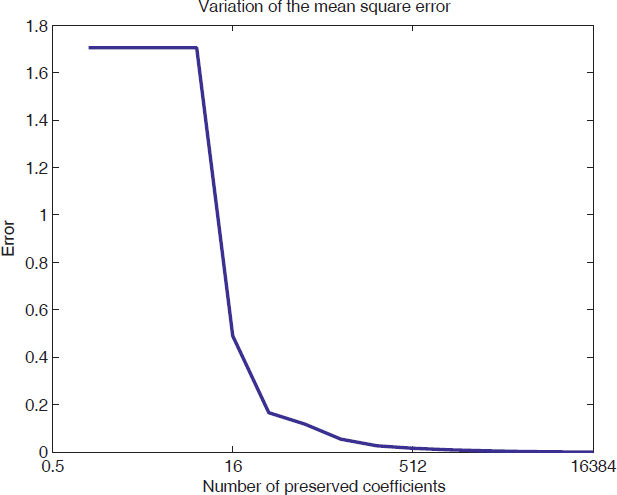
Figure 14.3. Variation of the mean square error (the horizontal axis is represented in logarithmic scale)

b.

load imdemos dots r=1024; [N1,N2]=size(dots); sl=double(dots); s=zeros(N1,N2); s=sl; y=dct2(s); [ly,cy]=size(y); yv=y(:); [yvs,idxs]=sort(abs(yv)); yvs=flipud(yvs); idxs=flipud(idxs); cont=0; yv(idxs(r+1:N1*N2))=zeros(N1*N2-r,1); for ...