6.3. Exercises
EXERCISE 6.18.
Consider the following transfer functions:
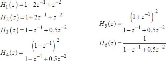
a. Plot the poles and zeros of these functions using the command zplane.m.
b. Represent the above transfer functions, using the command freqz.m, and indicate the type of corresponding systems.
c. Determine the indicial response of the system represented by H5(z).
EXERCISE 6.19.
A LTI1D is characterized by the following discrete-time equation:
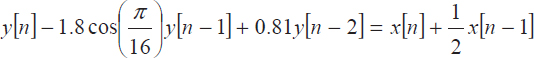
a. Determine the poles of the system transfer function which are the roots pk of the polynomial: 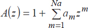 (use the MATLAB command roots.m). If these roots are complex conjugated, the system response will have the form of a complex exponential. Represent the real and imaginary parts of signals pnku[n].
b. As the transfer function of the system is of 2nd order, its impulse response has the form h[n] = (αp1n + βpn2)u[n]. Verify this statement using the system impulse response calculated using the MATLAB function impz.m
c. Find constants α and β from the expression of h[n].
d. Calculate the system stationary response to the complex exponential signal x[n] = ejπ/4n, n = 0..30, using the MATLAB function filter.m.
EXERCISE 6.20.
Consider the following transfer function:
a. Calculate and ...
Get Digital Signal Processing Using Matlab now with the O’Reilly learning platform.
O’Reilly members experience books, live events, courses curated by job role, and more from O’Reilly and nearly 200 top publishers.

