1.2. Solved exercises
EXERCISE 1.6.
Define a 4×3 matrix zero everywhere excepting the first line that is filled with 1.
b = ones (1, 3); m = zeros (4, 3); m(1, :) = b
m =
     1   1   1
     0   0   0
     0   0   0
     0   0   0
EXERCISE 1.7.
Consider the couples of vectors (x1 y1) and (x2, y2). Define the vector x so that:
x(j) = 0 if y1(j) <y2(j);
x(j) = x1(i) if y1(j) = y2(j);
x(j) = x2(j) if y1(j) > y2(j)
function x = vectors(x1,y1,x2,y2)
x = x1.*[y1 == y2] + x2.*[y1 > y2];

vectors ([0 1],[4 3], [-2 4] ,[2 0])

ans =
    -2 4
EXERCISE 1.8.
Generate and plot the signal: y(t) = sin(2πt) for 0 ≤ t ≤2, with an increment of 0.01, then undersample it (using the function decimate) with the factors 2 and 16.
t = 0:0.01:2;
y = sin(2*pi*t);
subplot(311)
plot(t,y) ;
ylabel('sin(2.pi.t)');
title('Original signal');
t2 = decimate(t, 2);
t16 = decimate(t2, 8);
y2 = decimate(y, 2);
y16 = decimate(y2, 8);
subplot(312) plot(t2, y2);
ylabel('sin(2.pi.t)')
title('Undersampled signal with a factor 2');
subplot(313);
plot(t16, y16);
ylabel('sin(2.pi.t)');
xlabel('Time t');
title('Undersampled signal with a factor 16');
You can save the figures in eps (Encapsulated PostScript) format, which is recognized by many software programs. The command print -eps file_name creates the file file_name.eps.
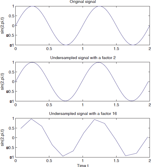
Figure 1.2. Sinusoid waveform corresponding to different sample frequencies
EXERCISE 1.9.
Plot the paraboloid defined by the equation: ...
Get Digital Signal Processing Using Matlab now with the O’Reilly learning platform.
O’Reilly members experience books, live events, courses curated by job role, and more from O’Reilly and nearly 200 top publishers.

