Chapter 4. Major Architectures of Deep Networks
The mother art is architecture. Without an architecture of our own we have no soul of our own civilization.
Frank Lloyd Wright
Now that we’ve seen some of the components of deep networks, let’s take a look at the four major architectures of deep networks and how we use the smaller networks to build them. Earlier in the book, we introduced four major network architectures:
- Unsupervised Pretrained Networks (UPNs)
- Convolutional Neural Networks (CNNs)
- Recurrent Neural Networks
- Recursive Neural Networks
In this chapter, we take a look in more detail at each of these architectures. In Chapter 2, we gave you a deeper understanding of the algorithms and math that underlie neural networks in general. In this chapter, we focus more on the higher-level architecture of different deep networks so as to build an understanding appropriate for applying these networks in practice.
Some networks we’ll cover more lightly than others, but we’ll mostly focus on the two major architectures that you will see in the wild: CNNs for image modeling and Long Short-Term Memory (LSTM) Networks (Recurrent Networks) for sequence modeling.
Unsupervised Pretrained Networks
In this group, we cover three specific architectures:
- Autoencoders
- Deep Belief Networks (DBNs)
- Generative Adversarial Networks (GANs)
A Note About the Role of Autoencoders
As we previously covered in Chapter 3, autoencoders fundamental structures in deep networks because they’re often used as part of larger networks. Like many other networks, they serve that role and then are used as a standalone network, as well.
Since we’ve already covered autoencoders in depth, we’ll move on to looking closer at DBNs and GANs.
Deep Belief Networks
DBNs are composed of layers of Restricted Boltzmann Machines (RBMs) for the pretrain phase and then a feed-forward network for the fine-tune phase. Figure 4-1 shows the network architecture of a DBN.
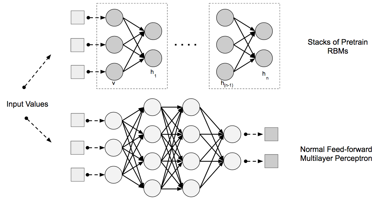
Figure 4-1. DBN architecture
In the sections that follow, we explain more about how DBNs take advantage of RBMs to better model training data.
Feature Extraction with RBM Layers
We use RBMs to extract higher-level features from the raw input vectors. To do that, we want to set the hidden unit states and weights such that when we show the RBM an input record and ask the RBM to reconstruct the record, it generates something pretty close to the original input vector. Hinton talks about this effect in terms of how machines “dream about data.”
The fundamental purpose of RBMs in the context of deep learning and DBNs is to learn these higher-level features of a dataset in an unsupervised training fashion. It was discovered that we could train better neural networks by letting RBMs learn progressively higher-level features using the learned features from a lower level RBM pretrain layer as the input to a higher-level RBM pretrain layer.
Learning higher-order features automatically
Learning these features in an unsupervised fashion is considered the pretrain phase of DBNs. Each hidden layer of the RBM in the pretrain phase learns progressively more complex features from the distribution of the data. These higher-order features are progressively combined in nonlinear ways to do elegant automated feature engineering.
To visually understand feature construction with layers of RRBMs, take a look at Figures 4-2, 4-3, and 4-4, which show the progression of activation renders on a RBM as it learns MNIST digits.
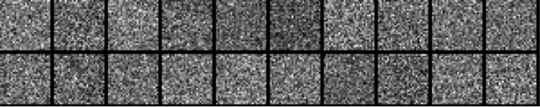
Figure 4-2. Activation render at the beginning of training
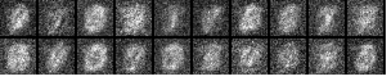
Figure 4-3. Features emerge in later activation render
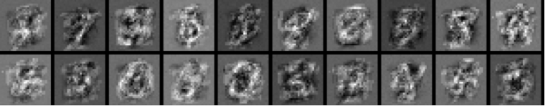
Figure 4-4. Portions of MNIST digits emerge towards end of training
Chapter 6 goes into more detail about how these renders are produced. We can see how a layer of RBM extracts fragments of digits as it trains. These features are then combined in higher-level layers to build progressively more complex (and nonlinear) features.
As this raw data is modeled in the generative modeling process with each layer of the RBM, the system is able to extract increasingly higher-level features from the raw input data produced by our baseline input vectorization process. These features move forward through these layers of RBMs in one direction, producing more elaborate features at the top layer.
Initializing the feed-forward network
We then use these layers of features as the initial weights in a traditional backpropagation driven feed-forward neural network.
These initialization values help the training algorithm guide the parameters of the traditional neural network toward better regions of parameter search space. This phase is known as the fine-tune phase of DBNs.
Fine-tuning a DBN with a feed-forward multilayer neural network
In the fine-tune phase of a DBN we use normal backpropagation with a lower learning rate to do “gentle” backpropagation. We consider the pretraining phase to be a general search of the parameter space in an unsupervised fashion based on raw data. In contrast, the fine-tune phase is about specializing the network and its features for the task we actually care about (such as classification).
Gentle backpropagation
The pretrain phase with RBM learns higher-order features from the data, which we use as good initial starting values for our feed-forward network. We want to take these weights and tune them a bit more to find good values for our final neural network model.
The output layer
The normal goal of a deep network is to learn a set of features. The first layer of a deep network learns how to reconstruct the original dataset. The subsequent layers learn how to reconstruct the probability distributions of the activations of the previous layer. The output layer of a neural network is tied to the overall objective. This is typically logistic regression, with the number of features equal to the number of inputs of the final layer, and the number of outputs equal to the number of classes.
Current state of DBNs
We don’t cover DBNs as extensively as the other network architectures in this book. This is because the field has largely seen CNNs take over the image modeling space and thus we chose to emphasize that architecture more, as you’ll see in the next section.
The Role of DBNs in the Rise of Deep Learning
Although we don’t emphasize DBNs as much in this book, this network played a nontrivial role in the rise of deep learning. Geoff Hinton’s team at the University of Toronto persisted over a long period of time in advancing techniques in the image modeling space to produce great advances. We felt it important to note the role that DBNs have played in the evolution of deep networks.
Generative Adversarial Networks
A network of note is the GAN.1 GANs have been shown to be quite adept at synthesizing novel new images based on other training images. We can extend this concept to model other domains such as the following:
GANs are an example of a network that uses unsupervised learning to train two models in parallel. A key aspect of GANs (and generative models in general) is how they use a parameter count that is significantly smaller than normal with respect to the amount of data on which we’re training the network. The network is forced to efficiently represent the training data, making it more effective at generating data similar to the training data.
Training generative models, unsupervised learning, and GANs
If we had a large corpus of training images (such as the ImageNet dataset), we could build a generative neural network that outputs images (as opposed to classifications). We’d consider these generated output images to be samples from the model. The generative model in GANs generates such images while a secondary “discriminator” network tries to classify these generated images.
This secondary discriminator network attempts to classify the output images as real or synthetic. When training GANs, we want to update the parameters such that the network will generate more believable output images based on the training data. The goal here is to make images realistic enough that the discriminator network is fooled to the point that it cannot distinguish the difference between the real and the synthetic input data.
An example of efficient model representation in GANs is how they typically have around 100 million parameters when modeling a dataset such as ImageNet. In the course of training, an input dataset such as ImageNet (200 GB) becomes close to 100 MB of parameters. This learning process tries to find the most efficient way to represent the features in the data, such as similar groups of pixels, edges, and other patterns (as we’ll see in more detail in “Convolutional Neural Networks (CNNs)”).
The discriminator network
When modeling images, the discriminator network is typically a standard CNN. Using a secondary neural network as the discriminator network allows the GAN to train both networks in parallel in an unsupervised fashion. These discriminator networks take images as input, and then output a classification.
The gradient of the output of the discriminator network with respect to the synthetic input data indicates how to make small changes to the synthetic data to make it more realistic.
The generative network
The generative network in GANs generates data (or images) with a special kind of layer called a deconvolutional layer (read more about deconvolutional networks and layers in the following sidebar).
During training, we use backpropagation on both networks to update the generating network’s parameters to generate more realistic output images. The goal here is to update the generating network’s parameters to the point at which the discriminating network is sufficiently “fooled” by the generating network because the output is so realistic as compared to the training data’s real images.
Building generative models and Deep Convolutional Generative Adversarial Networks
One variant of GANs is the Deep Convolutional Generative Adversarial Network (DCGAN). Figure 4-6 depicts images of bedrooms generated from a DCGAN.
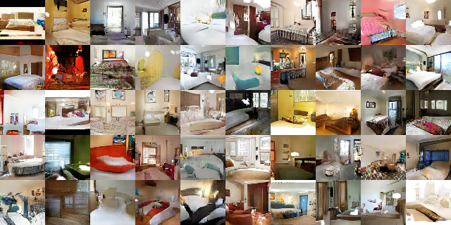
Figure 4-6. Generated images of bedrooms from a DCGAN network4
This network takes random numbers (from a uniform distribution) and generates an image from the network model as output. As the input random numbers change we see the DCGAN generate different types of images.
Conditional GANs
Conditional GANs5 also can use class label information, allowing them to conditionally generate data of a specific class.
Comparing GANs and variational autoencoders
GANs focus on trying to classify training records as being from the model distribution or the real distribution. When the discriminator model makes a prediction in which there is a difference between the two distributions, the generator network adjusts its parameters. Eventually the generator converges on parameters that reproduce the real data distribution, and the discriminator is unable to detect the difference.
With variational autoencoders (VAEs) we’re setting up this same problem with probabilistic graphical models to reconstruct the input in an unsupervised fashion, as seen previously in Chapter 3. VAEs attempt to maximize a lower bound on the log likelihood of the data such that the generated images look more and more real.
Another interesting difference between GANs and VAEs is how the images are generated. With basic GANs the image is generated with arbitrary code and we don’t have a way to generate a picture with specific features. VAEs, in contrast, have a specific encode/decode scheme with which we can compare the generated image to the original image. This gives us the side effect of being able to code for specific types of images to be generated.
Issues with Generative Models
Sometimes with generated images we also get a different type of noise in the generated output image. The downside of VAE-generated images is that as a result of how they are generated, the images are sometimes slightly blurry. GAN-generated images tend to capture the style of the input data yet sometimes don’t compose the scene in a coherent manner (e.g., it’s an image of a dog, but the dog doesn’t look quite right).
Convolutional Neural Networks (CNNs)
The goal of a CNN is to learn higher-order features in the data via convolutions. They are well suited to object recognition with images and consistently top image classification competitions. They can identify faces, individuals, street signs, platypuses, and many other aspects of visual data. CNNs overlap with text analysis via optical character recognition, but they are also useful when analyzing words6 as discrete textual units. They’re also good at analyzing sound.
The efficacy of CNNs in image recognition is one of the main reasons why the world recognizes the power of deep learning. As Figure 4-7 illustrates, CNNs are good at building position and (somewhat) rotation invariant features from raw image data.
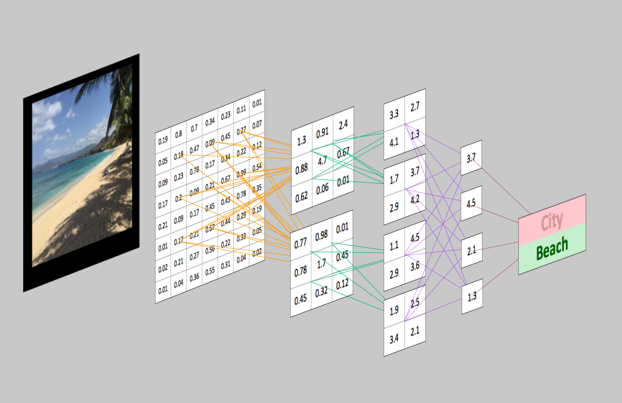
Figure 4-7. CNNs and computer vision
CNNs are powering major advances in machine vision, which has obvious applications for self-driving cars, robotics, drones, and treatments for the visually impaired.
CNNs and Structure in Data
CNNs tend to be most useful when there is some structure to the input data. An example would be how images and audio data that have a specific set of repeating patterns and input values next to each other are related spatially. Conversely, the columnar data exported from a relational database management system (RDBMS) tends to have no structural relationships spatially. Columns next to one another just happen to be materialized that way in the database exported materialized view.
CNNs also have been used in other tasks such as natural language translation/generation7 and sentiment analysis.8 A convolution is a powerful concept for helping to build a more robust feature space based on a signal.
Biological Inspiration
The biological inspiration for CNNs is the visual cortex in animals.9 The cells in the visual cortex are sensitive to small subregions of the input. We call this the visual field (or receptive field). These smaller subregions are tiled together to cover the entire visual field. The cells are well suited to exploit the strong spatially local correlation found in the types of images our brains process, and act as local filters over the input space. There are two classes of cells in this region of the brain. The simple cells activate when they detect edge-like patterns, and the more complex cells activate when they have a larger receptive field and are invariant to the position of the pattern.
Intuition
Feed-forward multilayer neural networks take input as a single one-dimensional vector and transform the data with one or more hidden layers (fully connected). The network then gives a result from the output layer. The issue we run into with traditional multilayer neural networks and image data is that these networks don’t scale well with image data as input. An example would be modeling the CIFAR-10 dataset (see the upcoming sidebar). The images to train on are only 32 pixels wide by 32 pixels in height with 3 channels of RGB information. This creates 3,072 weights per neuron in the first hidden layer, however, and we’ll probably want more than one neuron in that hidden layer. In many cases, we’ll want multiple hidden layers in our multilayer neural network, which will multiply those weights, as well.
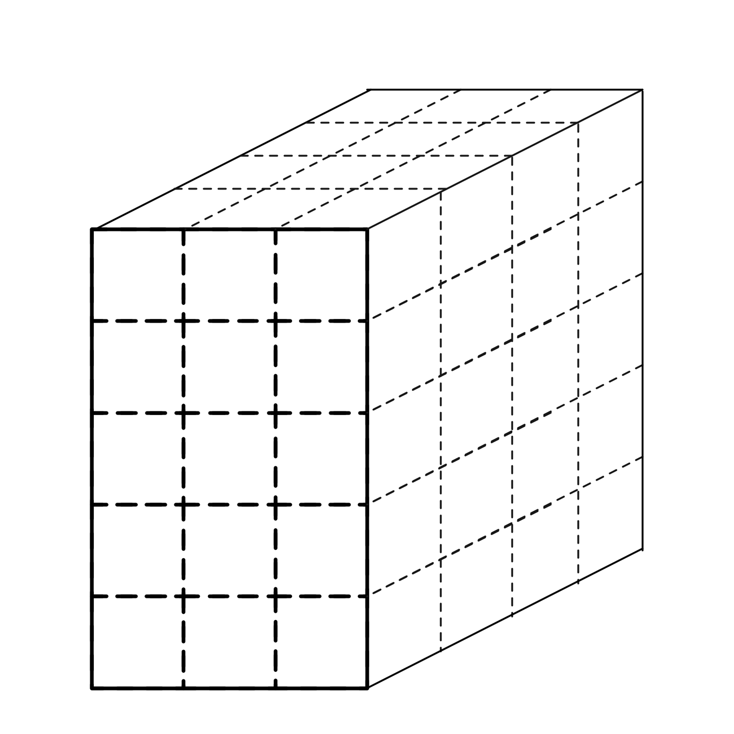
A normal image could easily be 300 pixels in width by 300 pixels in height with 3 channels of RGB information. This would create 270,000 connection weights per hidden neuron. This shows how quickly a fully connected multilayer network creates a massive number of connections when modeling image data. The structure of image data allows us to change the architecture of a neural network in a way that we can take advantage of this structure. With CNNs, we can arrange the neurons in a three-dimensional structure for which we have the following:
- Width
- Height
- Depth
These attributes of the input match up to an image structure for which we have:
- Image width in pixels
- Image height in pixels
- RGB channels as the depth
We can consider this structure to be a three-dimensional volume of neurons. A significant aspect to how CNNs evolved from previous feed-forward variants is how they achieved computational efficiency with new layer types. We’ll cover this arrangement in more depth momentarily. Let’s now take a look at the high-level general architecture of CNNs.
CNN Architecture Overview
CNNs transform the input data from the input layer through all connected layers into a set of class scores given by the output layer. There are many variations of the CNN architecture, but they are based on the pattern of layers, as demonstrated in Figure 4-9.
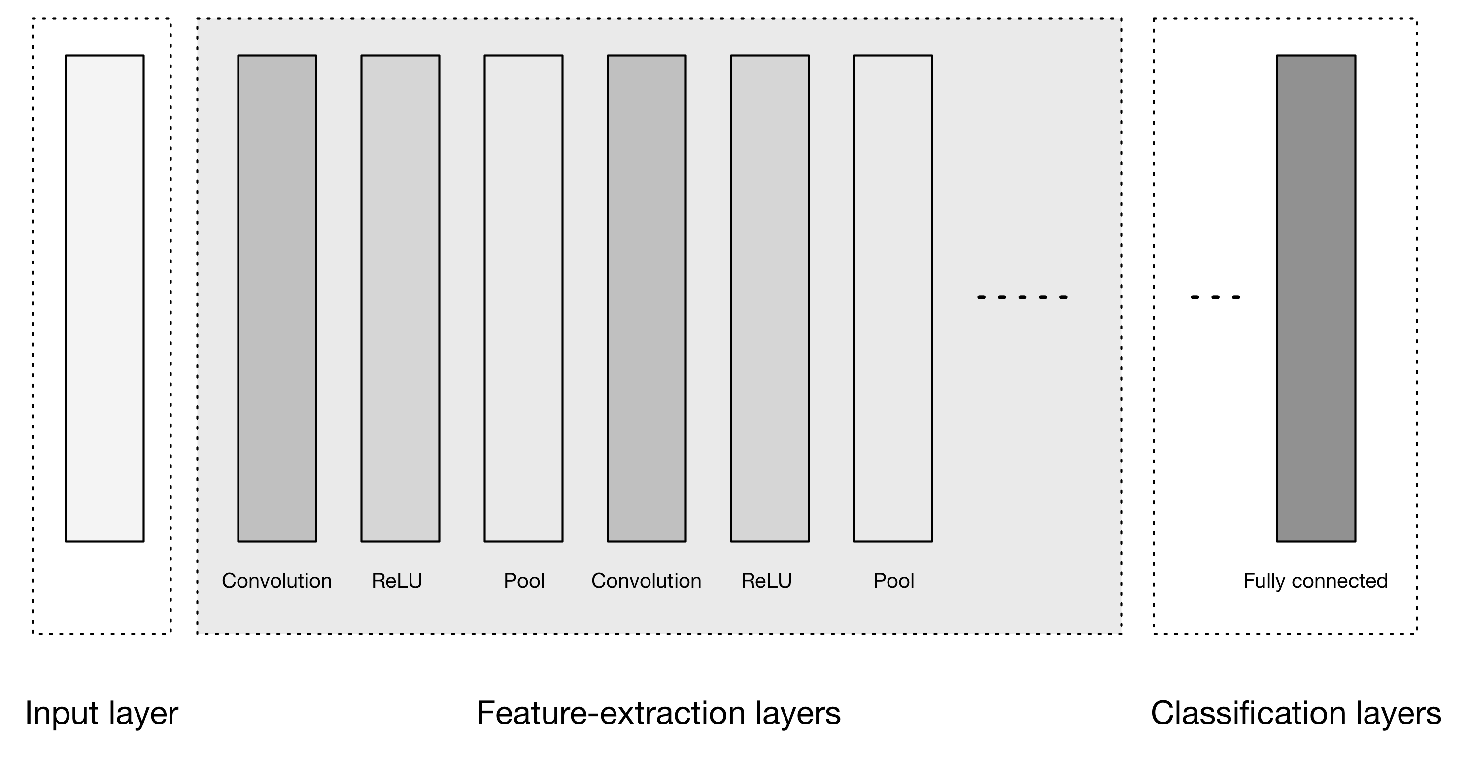
Figure 4-9. High-level general CNN architecture
Figure 4-9 depicts three major groups:
- Input layer
- Feature-extraction (learning) layers
- Classification layers
The input layer accepts three-dimensional input generally in the form spatially of the size (width × height) of the image and has a depth representing the color channels (generally three for RGB color channels).
Mini-Batch as the Fourth Dimension
When we batch examples together into a mini-batch for training, we end up with four dimensions—one more dimension to index the example within the mini-batch. Thus, in DL4J, image training data arrays have four dimensions, not just three.
The feature-extraction layers have a general repeating pattern of the sequence:
-
Convolution layer
We express the Rectified Linear Unit (ReLU) activation function as a layer in the diagram here to match up to other literature.
- Pooling layer
These layers find a number of features in the images and progressively construct higher-order features. This corresponds directly to the ongoing theme in deep learning by which features are automatically learned as opposed to traditionally hand engineered.
Finally we have the classification layers in which we have one or more fully connected layers to take the higher-order features and produce class probabilities or scores. These layers are fully connected to all of the neurons in the previous layer, as their name implies. The output of these layers produces typically a two-dimensional output of the dimensions [b × N], where b is the number of examples in the mini-batch and N is the number of classes we’re interested in scoring.
Neuron spatial arrangements
Recall how in traditional multilayer neural networks, the layers are fully connected and every neuron in a layer is connected to every neuron in the next layer. The neurons in the layers of a CNN are arranged in three dimensions to match the input volumes. Here, depth means the third dimension of the activation volume, not the number of layers, as in a multilayer neural network.
Evolution of the connections between layers
Another change is how we connect layers in a convolutional architecture. Neurons in a layer are connected to only a small region of neurons in the layer before it. CNNs retain a layer-oriented architecture, as in traditional multilayer networks, but have different types of layers. Each layer transforms the 3D input volume from the previous layer into a 3D output volume of neuron activations with some differentiable function that might or might not have parameters, as demonstrated in Figure 4-10.
Convolutional Layers
Convolutional layers are considered the core building blocks of CNN architectures. As Figure 4-11 illustrates, convolutional layers transform the input data by using a patch of locally connecting neurons from the previous layer. The layer will compute a dot product between the region of the neurons in the input layer and the weights to which they are locally connected in the output layer.
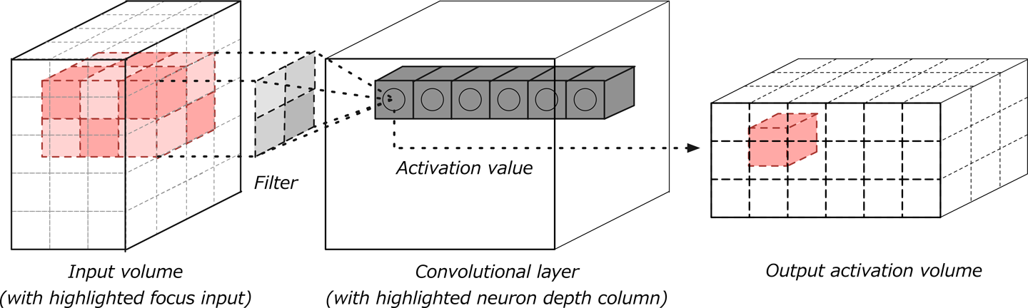
Figure 4-11. Convolution layer with input and output volumes
The resulting output generally has the same spatial dimensions (or smaller spatial dimensions) but sometimes increases the number of elements in the third dimension of the output (depth dimension). Let’s take a closer look at a key concept in these layers, called a convolution.
Convolution
A convolution is defined as a mathematical operation describing a rule for how to merge two sets of information. It is important in both physics and mathematics and defines a bridge between the space/time domain and the frequency domain through the use of Fourier transforms. It takes input, applies a convolution kernel, and gives us a feature map as output.
The convolution operation, shown in Figure 4-12, is known as the feature detector of a CNN. The input to a convolution can be raw data or a feature map output from another convolution. It is often interpreted as a filter in which the kernel filters input data for certain kinds of information; for example, an edge kernel lets pass through only information from the edge of an image.
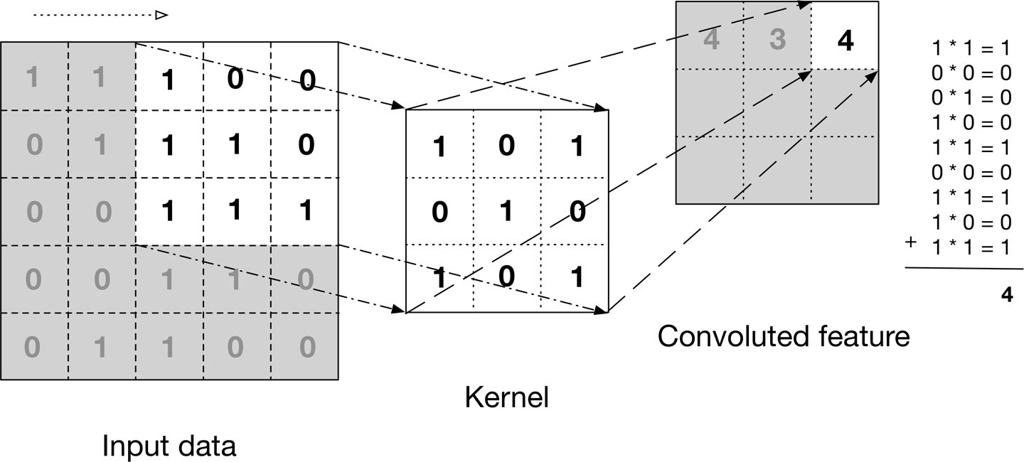
Figure 4-12. The convolution operation
The figure illustrates how the kernel is slid across the input data to produce the convoluted feature (output) data. At each step, the kernel is multiplied by the input data values within its bounds, creating a single entry in the output feature map. In practice the output is large if the feature we’re looking for is detected in the input.
We commonly refer to the sets of weights in a convolutional layer as a filter (or kernel). This filter is convolved with the input and the result is a feature map (or activation map). Convolutional layers perform transformations on the input data volume that are a function of the activations in the input volume and the parameters (weights and biases of the neurons). The activation map for each filter is stacked together along the depth dimension to construct the 3D output volume.
Convolutional layers have parameters for the layer and additional hyperparameters. Gradient descent is used to train the parameters in this layer such that the class scores are consistent with the labels in the training set. Following are the major components of convolutional layers:
- Filters
- Activation maps
- Parameter sharing
- Layer-specific hyperparameters
Let’s take a look of the specifics of each component.
Filters
The parameters for a convolutional layer configure the layer’s set of filters. Filters are a function that has a width and height smaller than the width and height of the input volume.
Filter Sizes in Natural Language Processing Applications
We can have a filter size equal to the input volume, but typically only in one dimension, not both. This would be something to be aware of for cases in which we’d apply CNNs to use cases in Natural Language Processing (NLP).
Filters (e.g., convolutions) are applied across the width and height of the input volume in a sliding window manner, as demonstrated in Figure 4-12. Filters are also applied for every depth of the input volume. We compute the output of the filter by producing the dot product of the filter and the input region.
Filter Count and Activation Maps
The output of applying a filter to the input volume is known as the activation map (sometimes referred to as a feature map) of that filter. In many CNN diagrams, we often see lots of small activation maps; how these are produced can sometimes be confusing.
The filter count is a hyperparameter value for each convolutional layer. This hyperparameter also controls how many activation maps are produced from the convolutional layer as input into the next layer and is considered the third dimension (number of activation maps) in the 3D layer output activation volume. The filter count hyperparameter can be chosen freely yet some values will work better than others.
The architecture of CNNs is set up such that the learned filters produce the strongest activation to spatially local input patterns. This means that filters are learned that will activate on patterns (or features) only when the patterns occur in the training data in their respective field. As we move farther along in layers in a CNN, we encounter filters that can recognize nonlinear combinations of features and are increasingly global in how they can detect patterns. High-performing convolutional architectures (which we’ll see later in this section) have shown network depth to be an important factor in CNNs.
Activation maps
Recall from Chapter 1 that an activation is a numerical result if a neuron decided to let information pass through. This is a function of the inputs to the activation function, the weights on the connections (for the inputs, and the type of activation function itself). When we say the filter “activates,” we mean that the filter lets information pass through it from the input volume into the output volume.
We slide each filter across the spatial dimensions (width, height) of the input volume during the forward pass of information through the CNN. This produces a two-dimensional output called an activation map for that specific filter. Figure 4-13 depicts how this activation map relates to our previously introduced concept of a convoluted feature.
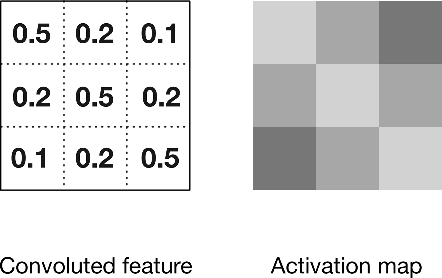
Figure 4-13. Convolutions and activation maps
The activation map on the right in Figure 4-13 is rendered differently to illustrate how convolutional activation maps are commonly rendered in the literature.
Activation Maps
In some literature, the activation map output is called a feature map, but for this text, we’ll refer to it as an activation map.
To compute the activation map, we slide the filter across the input volume depth slice. We calculate the dot product between the entries in the filter and the input volume. The filter represents the weights that are being multiplied by the moving window (subset) of input activations. Networks learn filters that activate when they see certain types of features in the input data in a specific spatial position.
We create the three-dimensional output volume for the convolution layer by stacking these activation maps along the depth dimension in the output, as shown in Figure 4-14. The output volume will have entries that we consider the output of a neuron that look at only a small window of the input volume.
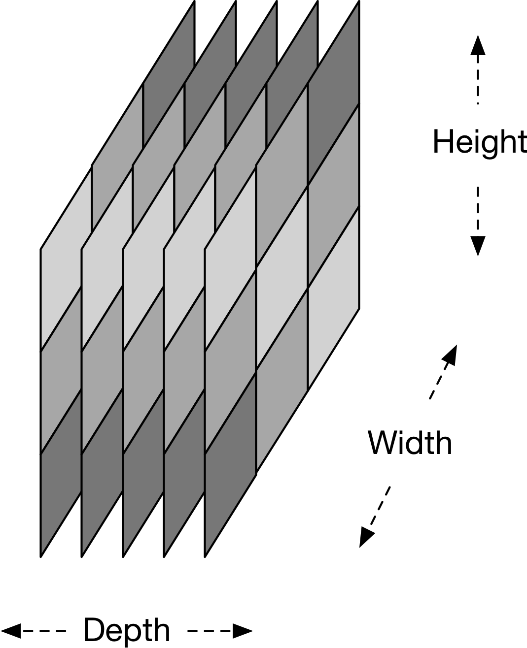
Figure 4-14. Activation volume output of convolutional layer
In some cases, this output will be the result of parameters shared with neurons in the same activation map. Each neuron generating the output volume is connected to only a local region of the input volume, as depicted in Figure 4-15.
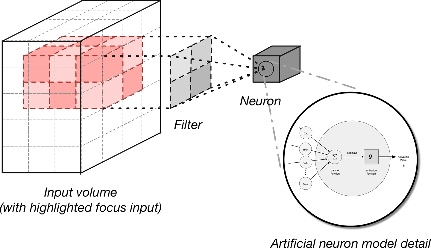
Figure 4-15. Generating an activation output volume
We control local connectivity of this process with the hyperparameter called the receptive field, which controls how much of the width and height of the input volume against which our filter maps.
Filters define a smaller bounded region to generate activation maps from the input volumes. They are connected to only a subset of the input volume through the dynamics of local connectivity described earlier. This allows us to still have quality feature extraction while reducing the number of parameters per layer we need to train. Convolutional layers reduce the parameter count further by using a technique called parameter sharing.
Parameter sharing
CNNs use a parameter-sharing scheme to control the total parameter count. This helps training time because we’ll use fewer resources to learn the training dataset. To implement parameter sharing in CNNs, we first denote a single two-dimensional slice of depth as a “depth slice.” We then constrain the neurons in each depth slice to use the same weights and bias. This gives us significantly fewer parameters (or weights) for a given convolutional layer.
We are not able to take advantage of parameter sharing when the input images we’re training on have a specific centered structure. We see this effect in faces when we always expect a specific feature to appear in a specific place (for centered faces). In this case we’d probably not use parameter sharing. Parameter sharing is what gives CNNs invariance to translation/position, as well.
Learned filters and renders
Figure 4-16 presents an example of the learned 96 filters of size 11 × 11 × 3. With the parameter-sharing scheme, we see that detecting a horizontal edge is useful in many places in the image due to the translationally invariant nature of images. This means that we’re able to learn the horizontal edge in one place and then not worry about learning it as a feature in all positions in the image.
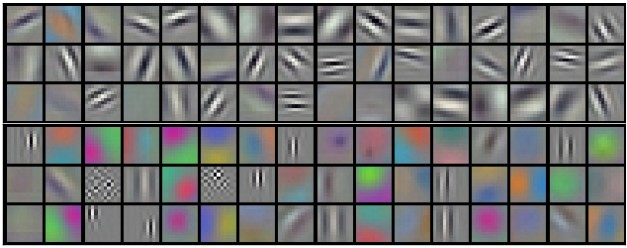
Figure 4-16. Example filters learned by Krizhevsky et al.10 (96 filters, 11 × 11 × 3)
Breaking this up a bit, let’s think about a 2D image. If we subdivide an image into four sections, the neural network will then learn position-invariant features of the image. The reason these are position invariant is because of how the network subdivides the data into quadrants. It then learns portions of the image at a time and pools the results. This allows the neural network to learn an overall representation that isn’t local to any particular set of features. We’ll talk more about generating filter renders in Chapter 6.
ReLU activation functions as layers
With CNNs, we often see ReLU layers used. The ReLU layer will apply an element-wise activation function over the input data thresholding—for example, max(0,x)—at zero, giving us the same dimension output as the input to the layer.
DL4J, layer types, and activation functions
In DL4J, we identify layers with their neuron activation function type (but this is not always reflected in the layer class names). DL4J has activation functions built into the layers themselves. Other libraries such as Caffe use separate activation layers.
Running this function over the input volume will change the pixel values but will not change the spatial dimensions of the input data in the output. ReLU layers do not have parameters nor additional hyperparameters.
Convolutional layer hyperparameters
Following are the hyperparameters11 that dictate the spatial arrangement and size of the output volume from a convolutional layer are:
- Filter (or kernel) size (field size)
- Output depth
- Stride
- Zero-padding
More on Sizing Convolutional Layers in Chapter 7
In this section, we explain how these hyperparameters work. In Chapter 7, we lay out the tuning mechanics for CNN layers.
Filter size
Every filter is small spatially with respect to the width and height of the filter size. An example of this is how the first convolutional layer might have a 5 × 5 × 3-sized filter. This would mean the filter is 5 pixels wide by 5 pixels tall, with 3 representing the color channels, assuming that the input image was in 3-channel RGB color.
Output depth
We can manually pick the depth of the output volume. The depth hyperparameter controls the neuron count in the convolutional layer that is connected to the same region of the input volume.
Edges and Activation
Different neurons along the depth dimension learn to activate when stimulated with created input data (e.g., color or edges).
We consider a set of neurons that all look at the same region of input volume as a depth column.
Stride
Stride configures how far our sliding filter window will move per application of the filter function. Each time we apply the filter function to the input column, we create a new depth column in the output volume. Lower settings for stride (for example, 1 specifies only a single unit step) will allocate more depth columns in the output volume. This also will yield more heavily overlapping receptive fields between the columns, leading to larger output volumes. The opposite is true when we specify higher stride values. These higher stride values give us less overlap and smaller output volumes spatially.
Batch normalization and layers
To accelerate training in CNNs we can normalize the activations of the previous layer at each batch.12 This technique applies a transformation that keeps the mean activation close to 0.0 while also keeping the activation standard deviation close to 1.0.
Batch normalization in CNNs has shown to speed up training by making normalization part of the network architecture. By applying normalization for each training mini-batch of input records, we can use much higher learning rates. Batch normalization also reduces the sensitivity of training toward weight initialization and acts as a regularizer (reducing the need for other types of regularization). Batch normalization has also been applied to LSTM networks,13 which is another type of deep network we’ll discuss later in the chapter.
Pooling Layers
Pooling layers are commonly inserted between successive convolutional layers. We want to follow convolutional layers with pooling layers to progressively reduce the spatial size (width and height) of the data representation. Pooling layers reduce the data representation progressively over the network and help control overfitting. The pooling layer operates independently on every depth slice of the input.
Common Downsampling Operations
The most common downsampling operation is the max operation. The next most common operation is average pooling.
The pooling layer uses the max() operation to resize the input data spatially (width, height). This operation is referred to as max pooling. With a 2 × 2 filter size, the max() operation is taking the largest of four numbers in the filter area. This operation does not affect the depth dimension.
Pooling layers use filters to perform the downsampling process on the input volume. These layers perform downsampling operations along the spatial dimension of the input data. This means that if the input image were 32 pixels wide by 32 pixels tall, the output image would be smaller in width and height (e.g., 16 pixels wide by 16 pixels tall). The most common setup for a pooling layer is to apply 2 × 2 filters with a stride of 2. This will downsample each depth slice in the input volume by a factor of two on the spatial dimensions (width and height). This downsampling operation will result in 75 percent of the activations being discarded.
Pooling layers do not have parameters for the layer but do have additional hyperparameters. This layer does not involve parameters, because it computes a fixed function of the input volume. It is not common to use zero-padding for pooling layers.
Fully Connected Layers
We use this layer to compute class scores that we’ll use as output of the network (e.g., the output layer at the end of the network). The dimensions of the output volume is [ 1 × 1 × N ], where N is the number of output classes we’re evaluating. In the case of the CIFAR dataset we discussed above, N would be 10 for the 10 classes of objects in the dataset. This layer has a connection between all of its neurons and every neuron in the previous layer.
Fully connected layers have the normal parameters for the layer and hyperparameters. Fully connected layers perform transformations on the input data volume that are a function of the activations in the input volume and the parameters (weights and biases of the neurons).
Multiple Fully Connected Layers
There are some CNN architectures that will use multiple fully connected layers at the end of the network. AlexNet is an example of this; it has two fully connected layers followed by a softmax layer at the end.
Other Applications of CNNs
Beyond normal two-dimensional image data, we also see CNNs applied to three-dimensional datasets. Here are some examples of these alternative uses:
The position-invariant nature of CNNs has proven useful in these domains because we’re not limited to hand-coding our features to appear in certain “spots” in the feature vector.
Summary
CNNs evolved due to the need for specialized feature extraction from image data. We saw layers that are good at finding features no matter where they “roam” across columns. We saw how convolutional layers, pooling layers, and regular fully connected layers worked together to do image classification. Now, let’s move on to a neural network architecture focused on modeling the temporal domain: Recurrent Neural Networks.
Recurrent Neural Networks
Recurrent Neural Networks are in the family of feed-forward neural networks. They are different from other feed-forward networks in their ability to send information over time-steps. Here’s an interesting explanation of Recurrent Neural Networks from leading researcher Juergen Schmidhuber:
[Recurrent Neural Networks] allow for both parallel and sequential computation, and in principle can compute anything a traditional computer can compute. Unlike traditional computers, however, Recurrent Neural Networks are similar to the human brain, which is a large feedback network of connected neurons that somehow can learn to translate a lifelong sensory input stream into a sequence of useful motor outputs. The brain is a remarkable role model as it can solve many problems current machines cannot yet solve.
Historically, these networks have been difficult to train, but more recently, advances in research (optimization, network architectures, parallelism, and graphics processing units [GPUs]) have made them more approachable for the practitioner.
Recurrent Neural Networks take each vector from a sequence of input vectors and model them one at a time. This allows the network to retain state while modeling each input vector across the window of input vectors. Modeling the time dimension is a hallmark of Recurrent Neural Networks.
Modeling the Time Dimension
Recurrent Neural Networks are considered Turing complete and can simulate arbitrary programs (with weights). If we view neural networks as optimization over functions, we can consider Recurrent Neural Networks as “optimization over programs.” Recurrent neural networks are well suited for modeling functions for which the input and/or output is composed of vectors that involve a time dependency between the values. Recurrent neural networks model the time aspect of data by creating cycles in the network (hence, the “recurrent” part of the name).
Lost in time
Many classification tools (support vector machines, logistic regression, and regular feed-forward networks) have been applied successfully without modeling the time dimension, assuming independence. Other variations of these tools capture the time dynamic by modeling a sliding window of the input (e.g., the previous, current, and next input together as a single input vector).
A drawback of these tools is that assuming independence in the time connection between model inputs does not allow our model to capture long-range time dependencies. Sliding window techniques have a limited window width and will fail to capture any effects larger than the fixed window size. A great example of this is modeling how conversations work and having machines understand how to reply in a coherent fashion as the conversation evolves over time. A well-trained Recurrent Neural Network could compete in Alan Turing’s famed Turing Test, for instance, which attempts to fool a human into thinking he is speaking with a real person.
Temporal feedback and loops in connections
Recurrent Neural Networks can have loops in the connections. This allows them to model temporal behavior gain accuracy in domains such as time-series, language, audio, and text.
A Note About Connections from Output to Hidden Layers
In practice, we see this connectivity scheme less often than others. DL4J does not use this scheme either. We felt it important to note this variant, however, for context in the material. Most often we see connections between neurons in one time step to the next in each recurrent layer.
Data in these domains are inherently ordered and context sensitive where later values depend on previous ones. The wiring for a Recurrent Neural Network allows for feedback in ways that make it possible to capture these temporal effects. We primarily see Recurrent Neural Network architectures applied in the time-series domains for applications.
A Recurrent Neural Network includes a feedback loop that it uses to learn from sequences, including sequences of varying lengths. Recurrent Neural Networks contain an extra parameter matrix for the connections between time-steps, which are used/trained to capture the temporal relationships in the data.
Recurrent Neural Networks are trained to generate sequences, in which the output at each time-step is based on both the current input and the input at all previous time steps. Normal Recurrent Neural Networks compute a gradient with an algorithm called backpropagation through time (BPTT). We go into detail about BPTT later in the chapter.
Sequences and time-series data
We find sequential data in many problem domains in industry for which our model needs to output a sequence of vectors:
- Image captioning
- Speech synthesis24
- Music generation25
- Playing video games
- Language modeling
- Character-level text generation models
In other domains, we need a sequence of input vectors:
- Time-series prediction
- Video analysis
- Music information retrieval
And then we have domains that require both a series of input and output vectors:
- Natural language translation26
- Engaging in dialogue
- Robotic control
Recurrent Neural Networks contrast with other deep networks in what type of input they can model (nonfixed input):
- Nonfixed computation steps
- Nonfixed output size
- It can operate over sequences of vectors, such as frames of video
An important facet of Recurrent Neural Networks is how we can work with input and output in unique ways.
Understanding model input and output
Traditional machine learning operates on the concept of a single fixed-sized input vector. In traditional modeling activities, we typically would see an input-to-output relationship of fixed input size to fixed output size.
This is commonly the pattern for modeling in building classifiers for image classification or classifying columnar data.
Recurrent Neural Networks change this input dynamic to include multiple input vectors, one for each time-step, and each vector can have many columns. The following list gives examples of how Recurrent Neural Networks operate on sequences of input and output vectors:
- One-to-many: sequence output. For example, image captioning takes an image and outputs a sequence of words.
- Many-to-one: sequence input. For example, sentiment analysis where a given sentence is input.
- Many-to-many: For example, video classification: label each frame.
Now that we’ve looked at variations of input and output data, let’s take a look at how these input data are represented.
3D Volumetric Input
Input into Recurrent Neural Networks involves more dimensions than standard machine learning modeling input. This is similar conceptually to CNNs. We have three dimensions for the input:
- Mini-batch Size
- Number of columns in our vector per time-step
- Number of time-steps
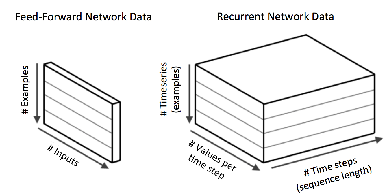
Figure 4-17. Normal input vectors compared to recurrent neural networks input
Mini-batch size is the number of input records (collections of time-series points for a single source entity) we want to model per batch. The number of columns matches up to the traditional feature column count found in a normal input vector. The number of time-steps is how we represent the change in the input vector over time. This is the time-series aspect to the input data. In the terminology from the previous section, we’d consider any time-step count above 1 to be “many-to-” in terms of input and output architecture.
Uneven time-series and masking
We previously described how with Recurrent Neural Network input we have the concept of time-steps in addition to features in our input vector. Figure 4-18 provides a visual representation.
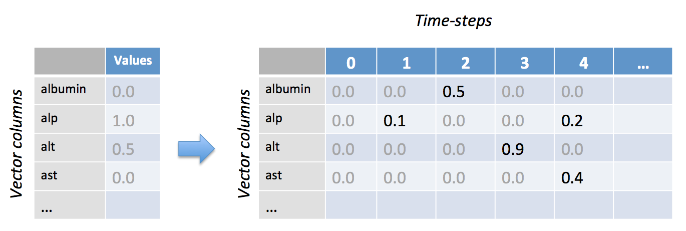
Figure 4-18. The time-step aspect of Recurrent Neural Network input
Every column value likely will not occur at every time-step, especially for the case in which we’re mixing descriptor data (e.g., columns from a static database table) with time-series data (e.g., measurements of an ICU patient’s heartrate every minute). For cases in which we have “jagged” time-step values, we need to use masking to let DL4J know where our real data is located in the vector. We do this by providing an extra matrix for the mask indicating the time-steps that have input data for at least one column, as demonstrated in Figure 4-19.
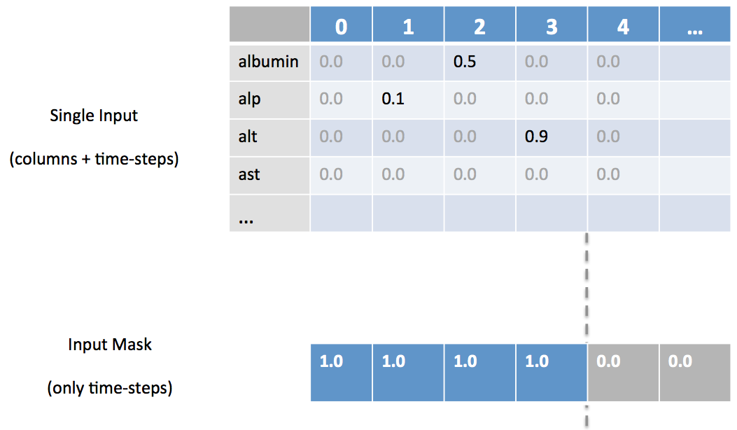
Figure 4-19. Masking specific time-steps
Chapter 3 provides real code examples that show how we set up these masks.
Why Not Markov Models?
When dealing with the time dimension in our models, we naturally could consider Markov models as an option. Markov models are another class of machine learning models that have been widely used for modeling sequences. The limiting factor with Markov models is that as their context window grows in size, eventually these models become computationally impractical for modeling long-range dependencies.
Recurrent Neural Networks (connectionist models) are better than Markov models (and other time-window limited models) because they can capture the long-range time dependencies in the input data. Recurrent Neural Networks accomplish this because their hidden state captures information from an arbitrarily long context window and does not have the limitation of the other techniques. Moreover, the number of states they can model is represented by the hidden layer of nodes, and these states grow exponentially with the number of nodes in the layer. This makes Recurrent Neural Networks exceptional at capturing a lot of time-dimension relevant information across many input vectors.
General Recurrent Neural Network Architecture
Recurrent Neural Networks are a superset of feed-forward neural networks but they add the concept of recurrent connections. These connections (or recurrent edges) span adjacent time-steps (e.g., a previous time-step), giving the model the concept of time. The conventional connections do not contain cycles in recurrent neural networks. However, recurrent connections can form cycles including connections back to the original neurons themselves at future time-steps.
Recurrent Neural Networks architecture and time-steps
At each time-step of sending input through a recurrent network, nodes receiving input along recurrent edges receive input activations from the current input vector and from the hidden nodes in the network’s previous state.
The output is computed from the hidden state at the given time-step. The previous input vector at the previous time step can influence the current output at the current time-step through the recurrent connections.
We can chain layers of these specialized recurrent neurons together to build better models. We connect the output of the previous layer to the input of the next layer similar to how we’d connect feed-forward multilayer neural networks.
LSTM Networks
LSTM networks are the most commonly used variation of Recurrent Neural Networks. LSTM networks were introduced in 1997 by Hochreiter and Schmidhuber.27
The critical component of the LSTM28 is the memory cell and the gates (including the forget gate,29 but also the input gate). The contents of the memory cell are modulated by the input gates and forget gates.30 Assuming that both of these gates are closed, the contents of the memory cell will remain unmodified between one time-step and the next. The gating structure allows information to be retained across many time-steps, and consequently also allows gradients to flow across many time-steps. This allows the LSTM model to overcome the vanishing gradient problem that occurs with most Recurrent Neural Network models.
Properties of LSTM networks
LSTMs are known for the following:
- Better update equations
- Better backpropagation
Here are some example use cases of LSTMs:
- Generating sentences (e.g., character-level language models)
- Classifying time-series
- Speech recognition
- Handwriting recognition
- Polyphonic music modeling
LSTM and Bidirectional Recurrent Neural Networks (BRNN) architectures have shown industry-leading benchmarks in recent years on tasks such as the following:
- Image captioning
- Language translation
- Handwriting recognition
LSTM networks consist of many connected LSTM cells and perform well in how efficient they are during learning.
A Note About Training Complexity in LSTMs
The computational complexity of the forward and backward pass operations scale linearly with the number of time-steps in the input sequence.
In the following sections, we provide an overview of the architecture and components of the LSTM.
LSTM network architecture
To better understand the complex arrangement of connections between units and layers in LSTM networks, let’s build on some earlier concepts.
Earlier in this book, we developed the concept of the feed-forward multilayer neural network, as depicted in Figure 4-20.
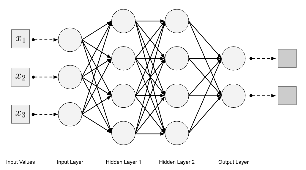
Figure 4-20. Feed-forward multilayer neural network architecture
If we were to show each layer from the network shown in Figure 4-20 as a single node in a flattened representation, it would look like Figure 4-21.
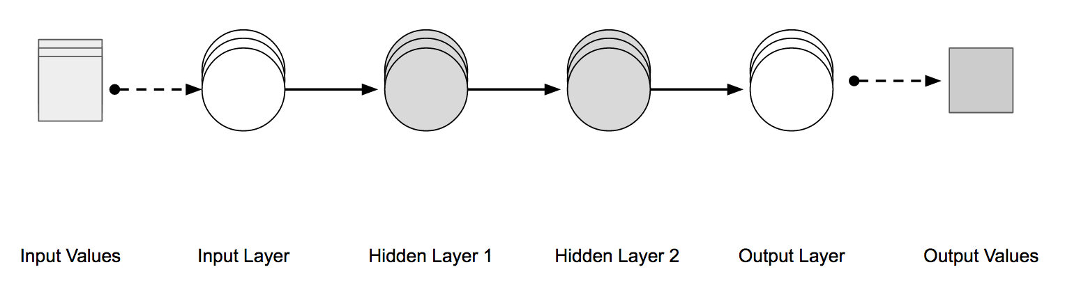
Figure 4-21. Visually feed-forward multilayer network
With Recurrent Neural Networks, we introduce the idea of a type of connection that connects the output of a hidden-layer neuron as an input to the same hidden-layer neuron. With this recurrent connection, we can take input from the previous time-step into the neuron as part of the incoming information.
Figure 4-22 demonstrates that by flattening the network shown in Figure 4-21, we can more easily visualize the recurrent connections in an LSTM.
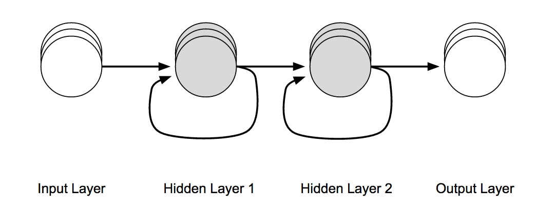
Figure 4-22. Showing recurrent connections on hidden-layer nodes
Figure 4-23 illustrates how we can further visually understand this by “unrolling” the network diagram in Figure 4-22 to show how the information “flows” through the network in a feed-forward manner and “across time.”
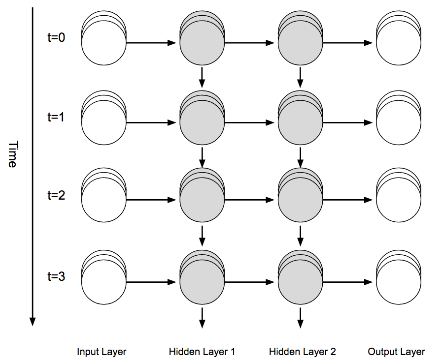
Figure 4-23. Recurrent Neural Network unrolled along the time axis
LSTM networks pass more information across the recurrent connection than the traditional Recurrent Neural Networks, as we’ll see in the next section.
LSTM units
The units in the layers of Recurrent Neural Networks are a variation on the classic artificial neuron.
Each LSTM unit has two types of connections:
- Connections from the previous time-step (outputs of those units)
- Connections from the previous layer
The memory cell in an LSTM network is the central concept that allows the network to maintain state over time. The main body of the LSTM unit is referred to as the LSTM block, as shown in Figure 4-24.
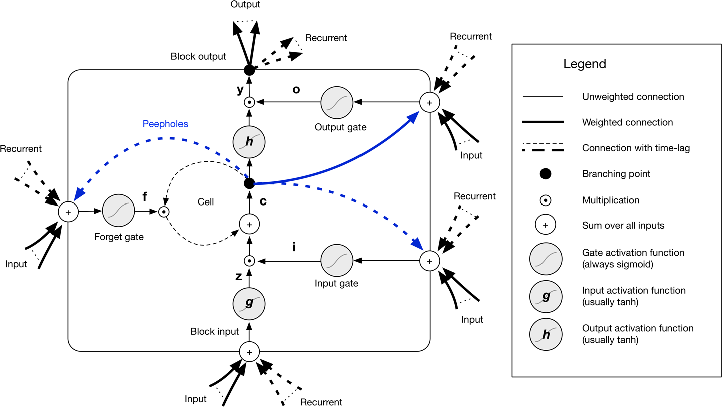
Figure 4-24. LSTM block diagram
Here are the components in an LSTM unit:
- Three gates
- input gate (input modulation gate)
- forget gate
- output gate
- Block input
- Memory cell (the constant error carousel)
- Output activation function
- Peephole connections
There are three gate units, which learn to protect the linear unit from misleading signals:
- The input gate protects the unit from irrelevant input events.
- The forget gate helps the unit forget previous memory contents.
- The output gate exposes the contents of the memory cell (or not) at the output of the LSTM unit.
The output of the LSTM block is recurrent connected back to the block input and all of the gates for the LSTM block. The input, forget, and output gates in an LSTM unit have sigmoid activation functions for [0, 1] restriction. The LSTM block input and output activation function (usually) is a tanh activation function.
A Note About the Forget Gate
An activation output of 1.0 means “remember everything” and activation output of 0.0 means “forget everything.” From a different perspective a better name for the forget gate might be the “remember gate”!
With this in mind we usually initialize the forget gate bias to a large value to enable learning of long-term dependencies (where large value == 1.0 by default in DL4J).
Using the notation from Greff et al.,31 Figure 4-25 presents the vector formulas for a LSTM layer forward pass.
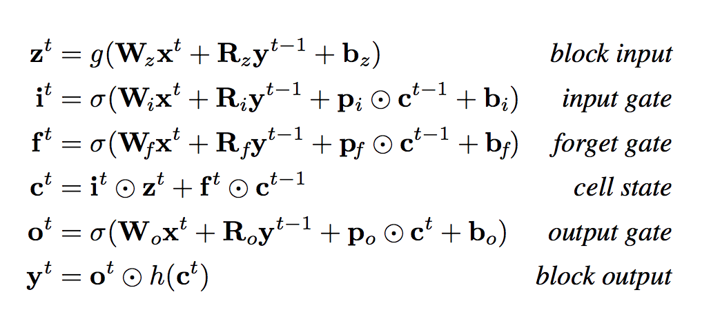
Figure 4-25. Vector formulas for LSTM layer forward pass
Table 4-1 lists the individual variables in the equations in Figure 4-25.
| Variable name | Description |
|---|---|
| xt | Input vector at time t |
| W | Rectangular input weight matrices |
| R | Square recurrent weight matrices |
| p | Peephole weight vectors |
| b | Bias vectors |
The self-recurrent connection has a fixed weight of 1.0 (except when modulated) to overcome issues with vanishing gradients. This core unit enables LSTM units to discover longer-range events in sequences. These events can span up to 1,000 discrete time-steps compared to older recurrent architectures, which could model events across around only 10 time-steps.
For More Variants of LSTMs...
Check out the paper “LSTM: A Search Space Odyssey.”
LSTM layers
A basic layer accepts an input vector x (nonfixed) and gives output y. The output y is influenced by the input x and the history of all inputs. The layer is influenced by the history of inputs through the recurrent connections. The RNN has some internal state that is updated every time we input a vector to the layer. The state consists of a single hidden vector.
Training
LSTM networks use supervised learning to update the weights in the network. They train on one input vector at a time in a sequence of vectors. Vectors are real-valued and become sequences of activations of the input nodes. Every noninput unit computes its current activation at any given time-step. This activation value is computed as the nonlinear function of the weighted sum of the activations of all units from which it receives connections.
For each input vector in the sequence of input, the error is equal to the sum of the deviations of all target signals from corresponding activations computed by the network. Let’s now take a look at the BPTT variant of backpropagation used with Recurrent Neural Networks, including LSTMs.
BPTT and truncated BPTT
Recurrent Neural Network training can be computationally expensive. The traditional option is to use BPTT.
Note
BPTT is fundamentally the same as standard backpropagation: we apply the chain rule to work out the derivatives (gradients) based on the connection structure of the network. It’s through time in the sense that some of those gradients/error signals will also flow backward from future time-steps to current time-steps, not just from the layer above (as occurs in standard backpropagation).
When our recurrent network is dealing with long sequences with many time-steps, we recommend alternatively using truncated BPTT. Truncated BPTT reduces the computational complexity of each parameter update in a Recurrent Neural Network.
Performing more frequent parameter updates speeds up recurrent neural network training. We recommend truncated BPTT when your input sequences are more than a few hundred time-steps.
To better understand the concepts involved with truncated BPTT, let’s consider what happens when we train a network with time-series input of length 12 (time-steps). In this scenario, we need to do a forward pass of 12 steps and then calculate the error of the network. Then, do a backward pass of the 12 time-steps, as demonstrated in Figure 4-26.
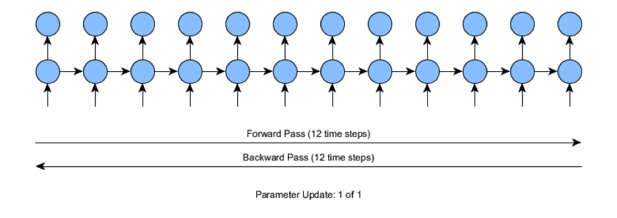
Figure 4-26. Standard BPTT
In the figure, the 12 time-steps are not that difficult for the training process. As we move into models that train on time-series data of a few hundred steps or more, we find training to be more difficult. If the number of steps in the time-series input were 1,000 steps, the standard backpropagation training would require 1,000 time-steps for each forward and backward pass (for each individual parameter update). This quickly becomes computationally expensive and is why we look at alternative training methods such as BPTT and truncated BPTT.
Truncated BPTT separates the forward and backward passes into smaller operations. The truncated BPTT shown in Figure 4-27 takes a smaller forward pass, makes an equally small backward pass, and then updates the intended parameter. This smaller pass size is a hyperparameter configured by the user. In the figure we can see that the truncated BPTT pass size is four time-steps.
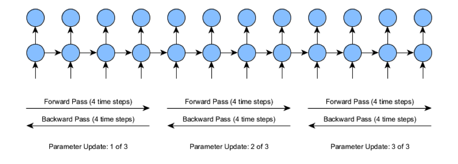
Figure 4-27. Truncated BPTT
Truncated BPTT is considered the current most practical method for training Recurrent Neural Networks. With truncated BPTT, we can capture long-term dependencies with less computational burden than regular BPTT.
The overall complexity for standard BPTT and truncated BPTT is similar and requires the same number of time-steps during training. However, we get more parameter updates for about the same amount of computational effort (although there is some overhead for each parameter update). As with all approximations, we see a slight downside when using truncated BPTT; the length of the dependencies learned in truncated BPTT can end up being shorter than the full BPTT algorithm’s results. In practice, this speed trade-off is generally worth it as long as truncated BPTT lengths are set correctly.
Domain-Specific Applications and Blended Networks
As mentioned earlier, Recurrent Neural Networks perform many domain-specific applications such as speech transcription to text, machine translation, and generation of handwritten text. Recurrent Neural Networks have proven to be adept in the world of computer vision and can do the following:
Another emerging area of research in computer vision with Recurrent Neural Networks is a network that can extract information from an image by processing only a small region at a time and is called Recurrent Models of Visual Attention.36 These models are effective at working with images that are cluttered with multiple objects and are more difficult for CNNs to classify. These networks blend together CNNs for raw perception and Recurrent Neural Networks for the time-domain modeling.
Another hybrid CNN + RNN network of note is the work by Andrej Karpathy and Li Fei-Fei, in which the network generates natural-language descriptions of images and their regions.37 The model is able to generate captions for images by using datasets of images and their corresponding sentence, as depicted in Figure 4-28.
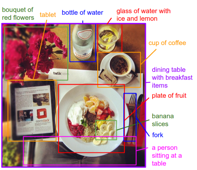
Figure 4-28. Labeling images with a blended CNN/Recurrent Neural Network38
Recursive Neural Networks
Recursive Neural Networks, like Recurrent Neural Networks, can deal with variable length input. The primary difference is that Recurrent Neural Networks have the ability to model the hierarchial structures in the training dataset. Images commonly have a scene composed of many objects. Deconstructing scenes is often a problem domain of interest yet is nontrivial. The recursive nature of this deconstruction challenges us to not only identify the objects in the scene, but also how the objects relate to form the scene.
Network Architecture
A Recursive Neural Network architecture is composed of a shared-weight matrix and a binary tree structure that allows the recursive network to learn varying sequences of words or parts of an image. It is useful as a sentence and scene parser. Recursive Neural Networks use a variation of backpropagation called backpropagation through structure (BPTS). The feed-forward pass happens bottom-up, and backpropagation is top-down. Think of the objective as the top of the tree, whereas the inputs are the bottom.
Varieties of Recursive Neural Networks
Recursive Neural Networks come in a few varieties. One is the recursive autoencoder. Just like its feed-forward cousin, recursive autoencoders learn how to reconstruct the input. In the case of NLP, it learns how to reconstruct contexts. A semisupervised recursive autoencoder learns the likelihood of certain labels in each context.
Another variation of this is a supervised neural network, called a Recursive Neural Tensor Network, which computes a supervised objective at each node of the tree. The tensor part of this means that it calculates the gradient a little differently, factoring in more information at each node by taking advantage of another dimension of information using a tensor (a matrix of three or more dimensions).
Applications of Recursive Neural Networks
Both Recursive and Recurrent Neural Networks share many of the same use cases. Recurrent Neural Networks are traditionally used in NLP because of their ties to binary trees, contexts, and natural-language-based parsers. For example, constituency parsers are able to break up a sentence into a binary tree, segmenting it by the linguistic properties of the sentence. In the case of Recursive Neural Networks, it is a constraint that we use a parser that builds the tree structure (typically constituency parsing).
Recursive Neural Networks can recover both granular structure and higher-level hierarchical structure in datasets such as images or sentences. Applications for recursive neural networks include the following:
- Image scene decomposition
- NLP
- Audio-to-text transcription
Two specific network configurations we see in practice are recursive autoencoders and recursive neural tensors. We use recursive autoencoders to break up sentences into segments for NLP. We use recursive neural tensors to break up an image into its composing objects and semantically label the objects in the scene.
Recurrent Neural Networks tend to be faster to train, thus we typically use them in more temporal applications, but they have been shown to work well in NLP-based domains such as sentiment analysis, as well.
Summary and Discussion
In this chapter, we reviewed the more recent major architectures in deep learning. In summary, to group and summarize these architectures, we note the following:
- To generate data (e.g., images, audio, or text), we’d use:
- GANs
- VAEs
- Recurrent Neural Networks
- To model images, we’d likely use:
- CNNs
- DBNs
- To model sequence data, we’d likely use:
- Recurrent Neural Networks/LSTMs
In the chapters that follow, we present real-world code examples of most of these networks and cover considerations of training and tuning for different kinds of neural networks. In Chapter 5 we see how these concepts come together in API examples in which we see the DL4J deep learning library in action. Before we move on to some more examples, let’s discuss a few topics that come up frequently in the context of deep learning.
Will Deep Learning Make Other Algorithms Obsolete?
The debate around deep learning making other modeling algorithms obsolete comes up many times on internet message boards. The answer today is “no” because for many simpler machine learning applications, we see far simpler algorithms work just fine for the required model accuracy. Models like logistic regression are also easier to work with, so we need to gauge the level of effort against the required accuracy in the domain when making this decision. However, deep learning algorithms tend to perform well when we understand little about the applied domain and struggle to do advanced handcrafted feature construction.
Different Problems Have Different Best Methods
Machine learning on the whole is about applying the correct approach in the appropriate situation. We’re not to the point yet where a single technique dominates the landscape so we need to evaluate the problem space and data each time we’re looking for the best model to apply. This is based on the “no free lunch theorem.”
No Free Lunch Theorem
The “no free lunch theorem” states that there is no one model that works for every problem. The assumptions for a great model for one problem might not hold for another problem. It is common in machine learning to try multiple models and find the one that works best for a particular problem.
Every machine learning method has some bias and variance. The closer our model is to the true underlying model the better we can do on average with our learning algorithm.
Another way to understand this is to consider it from the viewpoint of a practical example. If the data is clearly linear, as seen in visualizations, would you try and fit the data with a nonlinear model (e.g., a multilayer perceptron)? No, you’d probably approach the problem with something simpler, such as logistic regression. In Kaggle competitions, the method that performs best varies from competition to competition. However, random forests and ensemble methods tend to be the winners when deep learning does not win.
The input dataset size can be another factor in how appropriate deep learning can be for a given problem. Empirical results over the past few years have shown that deep learning provides the best predictive power when the dataset is large enough. This means deep learning results become better as dataset size increases. Neural networks have larger representational capacity than linear models and are better able to exploit the data. A nice rule of thumb is that a practitioner should be able to train a neural network with at least 5,000 training input labeled examples.
When Do I Need Deep Learning?
To close out this chapter, we want to leave you with a simple set of rules to help answer the question: does this project need to use deep learning?
When to use deep learning
You should use deep learning when...
- Simpler models (logistic regression) don’t achieve the accuracy level your use case needs
- You have complex pattern matching in images, NLP, or audio to deal with
- You have high dimensionality data
- You have the dimension of time in your vectors (sequences)
When to stick with traditional machine learning
You should use a traditional machine learning model when...
- You have high-quality, low-dimensional data; for example, columnar data from a database export
- You’re not trying to find complex patterns in image data
You’ll achieve poor results from both methods when the data is incomplete and/or of poor quality.
1 Goodfellow et al. 2014. “Generative Adversarial Networks.”
2 Vondrick, Pirsiavash, and Torralba. 2016. “Generating Videos with Scene Dynamics.”
3 Zhang et al. 2016. “StackGAN: Text to Photo-realistic Image Synthesis with Stacked Generative Adversarial Networks.”
4 Image is from the DCGAN authors’ GitHub repository.
5 Mirza and Osindero. 2014. “Conditional Generative Adversarial Nets.”
6 Kalchbrenner et al. 2016. “Neural Machine Translation in Linear Time.”
7 Gehring et al. 2016. “A Convolutional Encoder Model for Neural Machine Translation.”
8 Nogueira dos Santos and Gatti. 2014. “Deep Convolutional Neural Networks for Sentiment Analysis of Short Texts.”
9 Eickenberg et al. 2017. “Seeing it all: Convolutional network layers map the function of the human visual system.”
10 Krizhevsky et al. 2012. “ImageNet Classification with Deep Convolutional Neural Networks.”
11 Another hyperparameter commonly seen in CNNs is called dilation. DL4J currently does not support dilation as of version 0.7.
12 Ioffe and Szegedy. 2015. “Batch Normalization: Accelerating Deep Network Training by Reducing Internal Covariate Shift.”
13 Cooijmans et al. 2016. “Recurrent Batch Normalization.”
14 Milletari, Navab, and Ahmadi. 2016. “V-Net: Fully Convolutional Neural Networks for Volumetric Medical Image Segmentation.”
15 Maturana and Scherer. 2015. “VoxNet: A 3D Convolutional Neural Network for Real-Time Object Recognition.”
16 Henaff, Bruna, and LeCun. 2015. “Deep Convolutional Networks on Graph-Structured Data.”
17 Conneau et al. 2016. “Very Deep Convolutional Networks for Text Classification.”
18 LeCun et al. 1998. “Gradient-based learning applied to document recognition.”
19 Krizhevsky, Sutskever, and Hinton. 2012. “ImageNet Classification with Deep Convolutional Neural Networks.”
20 Zeiler and Fergus. 2013. “Visualizing and Understanding Convolutional Networks.”
21 Szegedy et al. 2015. “Going Deeper with Convolutions.”
22 Simonyan and Zisserman. 2015. “Very Deep Convolutional Networks for Large-Scale Image Recognition.”
23 He et al. 2015. “Deep Residual Learning for Image Recognition.”
24 Graves and Jaitly. 2014. “Towards End-to-End Speech Recognition with Recurrent Neural Network.”
25 Nayebi and Vitelli. 2015. “GRUV: Algorithmic Music Generation using Recurrent Neural Networks.”
26 Sutskever, Vinyals, and Le. 2014. “Sequence to Sequence Learning with Neural Networks.”
27 Hochreiter and Schmidhuber. 1997. “Long short-term memory.”
28 Graves. 2012. “Supervised Sequence Labelling with Recurrent Neural Networks.”
29 Gers, Schmidhuber, and Cummins. 1999. “Learning to Forget: Continual Prediction with LSTM.”
30 Graves. 2012. “Supervised Sequence Labelling with Recurrent Neural Networks.”
31 Greff et al. 2015. “LSTM: A Search Space Odyssey.”
32 Cho et al. 2014. “Learning Phrase Representations using RNN Encoder-Decoder for Statistical Machine Translation.”
33 Srivastava, Mansimov, and Salakhutdinov. 2015. “Unsupervised Learning of Video Representations using LSTMs.”
34 Venugopalan et al. 2014. “Translating Videos to Natural Language Using Deep Recurrent Neural Networks.”
35 Wu et al. 2016. “Image Captioning and Visual Question Answering Based on Attributes and External Knowledge.”
36 Mnih et al. 2014. “Recurrent Models of Visual Attention.”
37 Karpathy and Fei-Fei. 2014. “Deep Visual-Semantic Alignments for Generating Image Descriptions.”
38 The image is from Karpathy and Fei-Fei. 2014. “Deep Visual-Semantic Alignments for Generating Image Descriptions.”
Get Deep Learning now with the O’Reilly learning platform.
O’Reilly members experience books, live events, courses curated by job role, and more from O’Reilly and nearly 200 top publishers.

