Chapter 1. A Review of Machine Learning
To condense fact from the vapor of nuance
Neal Stephenson, Snow Crash
The Learning Machines
Interest in machine learning has exploded over the past decade. You see machine learning in computer science programs, industry conferences, and the Wall Street Journal almost daily. For all the talk about machine learning, many conflate what it can do with what they wish it could do. Fundamentally, machine learning is using algorithms to extract information from raw data and represent it in some type of model. We use this model to infer things about other data we have not yet modeled.
Neural networks are one type of model for machine learning; they have been around for at least 50 years. The fundamental unit of a neural network is a node, which is loosely based on the biological neuron in the mammalian brain. The connections between neurons are also modeled on biological brains, as is the way these connections develop over time (with “training”). We’ll dig deeper into how these models work over the next two chapters.
In the mid-1980s and early 1990s, many important architectural advancements were made in neural networks. However, the amount of time and data needed to get good results slowed adoption, and thus interest cooled. In the early 2000s computational power expanded exponentially and the industry saw a “Cambrian explosion” of computational techniques that were not possible prior to this. Deep learning emerged from that decade’s explosive computational growth as a serious contender in the field, winning many important machine learning competitions. The interest has not cooled as of 2017; today, we see deep learning mentioned in every corner of machine learning.
We’ll discuss our definition of deep learning in more depth in the section that follows. This book is structured such that you, the practitioner, can pick it up off the shelf and do the following:
- Review the relevant basic parts of linear algebra and machine learning
- Review the basics of neural networks
- Study the four major architectures of deep networks
- Use the examples in the book to try out variations of practical deep networks
We hope that you will find the material practical and approachable. Let’s kick off the book with a quick primer on what machine learning is about and some of the core concepts you will need to better understand the rest of the book.
How Can Machines Learn?
To define how machines can learn, we need to define what we mean by “learning.” In everyday parlance, when we say learning, we mean something like “gaining knowledge by studying, experience, or being taught.” Sharpening our focus a bit, we can think of machine learning as using algorithms for acquiring structural descriptions from data examples. A computer learns something about the structures that represent the information in the raw data. Structural descriptions are another term for the models we build to contain the information extracted from the raw data, and we can use those structures or models to predict unknown data. Structural descriptions (or models) can take many forms, including the following:
- Decision trees
- Linear regression
- Neural network weights
Each model type has a different way of applying rules to known data to predict unknown data. Decision trees create a set of rules in the form of a tree structure and linear models create a set of parameters to represent the input data.
Neural networks have what is called a parameter vector representing the weights on the connections between the nodes in the network. We’ll describe the details of this type of model later on in this chapter.
Arthur Samuel, a pioneer in artificial intelligence (AI) at IBM and Stanford, defined machine learning as follows:
[The f]ield of study that gives computers the ability to learn without being explicitly programmed.
Samuel created software that could play checkers and adapt its strategy as it learned to associate the probability of winning and losing with certain dispositions of the board. That fundamental schema of searching for patterns that lead to victory or defeat and then recognizing and reinforcing successful patterns underpins machine learning and AI to this day.
The concept of machines that can learn to achieve goals on their own has captivated us for decades. This was perhaps best expressed by the modern grandfathers of AI, Stuart Russell and Peter Norvig, in their book Artificial Intelligence: A Modern Approach:
How is it possible for a slow, tiny brain, whether biological or electronic, to perceive, understand, predict, and manipulate a world far larger and more complicated than itself?
This quote alludes to ideas around how the concepts of learning were inspired from processes and algorithms discovered in nature. To set deep learning in context visually, Figure 1-1 illustrates our conception of the relationship between AI, machine learning, and deep learning.
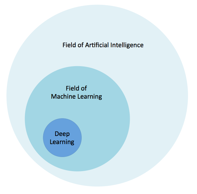
Figure 1-1. The relationship between AI and deep learning
The field of AI is broad and has been around for a long time. Deep learning is a subset of the field of machine learning, which is a subfield of AI. Let’s now take a quick look at another of the roots of deep learning: how neural networks are inspired by biology.
Biological Inspiration
Biological neural networks (brains) are composed of roughly 86 billion neurons connected to many other neurons.
Total Connections in the Human Brain
Researchers conservatively estimate there are more than 500 trillion connections between neurons in the human brain. Even the largest artificial neural networks today don’t even come close to approaching this number.
From an information processing point of view a biological neuron is an excitable unit that can process and transmit information via electrical and chemical signals. A neuron in the biological brain is considered a main component of the brain, spinal cord of the central nervous system, and the ganglia of the peripheral nervous system. As we’ll see later in this chapter, artificial neural networks are far simpler in their comparative structure.
Comparing Biological with Artificial
Biological neural networks are considerably more complex (several orders of magnitude) than the artificial neural network versions!
There are two main properties of artificial neural networks that follow the general idea of how the brain works. First is that the most basic unit of the neural network is the artificial neuron (or node in shorthand). Artificial neurons are modeled on the biological neurons of the brain, and like biological neurons, they are stimulated by inputs. These artificial neurons pass on some—but not all—information they receive to other artificial neurons, often with transformations. As we progress through this chapter, we’ll go into detail about what these transformations are in the context of neural networks.
Second, much as the neurons in the brain can be trained to pass forward only signals that are useful in achieving the larger goals of the brain, we can train the neurons of a neural network to pass along only useful signals. As we move through this chapter we’ll build on these ideas and see how artificial neural networks are able to model their biological counterparts through bits and functions.
What Is Deep Learning?
Deep learning has been a challenge to define for many because it has changed forms slowly over the past decade. One useful definition specifies that deep learning deals with a “neural network with more than two layers.” The problematic aspect to this definition is that it makes deep learning sound as if it has been around since the 1980s. We feel that neural networks had to transcend architecturally from the earlier network styles (in conjunction with a lot more processing power) before showing the spectacular results seen in more recent years. Following are some of the facets in this evolution of neural networks:
- More neurons than previous networks
- More complex ways of connecting layers/neurons in NNs
- Explosion in the amount of computing power available to train
- Automatic feature extraction
For the purposes of this book, we’ll define deep learning as neural networks with a large number of parameters and layers in one of four fundamental network architectures:
- Unsupervised pretrained networks
- Convolutional neural networks
- Recurrent neural networks
- Recursive neural networks
There are some variations of the aforementioned architectures—a hybrid convolutional and recurrent neural network, for example–as well. For the purpose of this book, we’ll consider the four listed architectures as our focus.
Automatic feature extraction is another one of the great advantages that deep learning has over traditional machine learning algorithms. By feature extraction, we mean that the network’s process of deciding which characteristics of a dataset can be used as indicators to label that data reliably. Historically, machine learning practitioners have spent months, years, and sometimes decades of their lives manually creating exhaustive feature sets for the classification of data. At the time of deep learning’s Big Bang beginning in 2006, state-of-the-art machine learning algorithms had absorbed decades of human effort as they accumulated relevant features by which to classify input. Deep learning has surpassed those conventional algorithms in accuracy for almost every data type with minimal tuning and human effort. These deep networks can help data science teams save their blood, sweat, and tears for more meaningful tasks.
Going Down the Rabbit Hole
Deep learning has penetrated the computer science consciousness beyond most techniques in recent history. This is in part due to how it has shown not only top-flight accuracy in machine learning modeling, but also demonstrated generative mechanics that fascinate even the noncomputer scientist. One example of this would be the art generation demonstrations for which a deep network was trained on a particular famous painter’s works, and the network was able to render other photographs in the painter’s unique style, as demonstrated in Figure 1-2.

Figure 1-2. Stylized images by Gatys et al., 20152
This begins to enter into many philosophical discussions, such as, “can machines be creative?” and then “what is creativity?” We’ll leave those questions for you to ponder at a later time. Machine learning has evolved over the years, like the seasons change: subtle but steady until you wake up one day and a machine has become a champion on Jeopardy or beat a Go Grand Master.
Can machines be intelligent and take on human-level intelligence? What is AI and how powerful could it become? These questions have yet to be answered and will not be completely answered in this book. We simply seek to illustrate some of the shards of machine intelligence with which we can imbue our environment today through the practice of deep learning.
For an Extended Discussion on AI
If you would like to read more about AI, take a look at Appendix A.
Framing the Questions
The basics of applying machine learning are best understood by asking the correct questions to begin with. Here’s what we need to define:
- What is the input data from which we want to extract information (model)?
- What kind of model is most appropriate for this data?
- What kind of answer would we like to elicit from new data based on this model?
If we can answer these three questions, we can set up a machine learning workflow that will build our model and produce our desired answers. To better support this workflow, let’s review some of the core concepts we need to be aware of to practice machine learning. Later, we’ll come back to how these come together in machine learning and then use that information to better inform our understanding of both neural networks and deep learning.
The Math Behind Machine Learning: Linear Algebra
Linear algebra is the bedrock of machine learning and deep learning. Linear algebra provides us with the mathematical underpinnings to solve the equations we use to build models.
Note
A great primer on linear algebra is James E. Gentle’s Matrix Algebra: Theory, Computations, and Applications in Statistics.
Let’s take a look at some core concepts from this field before we move on starting with the basic concept called a scalar.
Scalars
In mathematics, when the term scalar is mentioned, we are concerned with elements in a vector. A scalar is a real number and an element of a field used to define a vector space.
In computing, the term scalar is synonymous with the term variable and is a storage location paired with a symbolic name. This storage location holds an unknown quantity of information called a value.
Vectors
For our use, we define a vector as follows:
For a positive integer n, a vector is an n-tuple, ordered (multi)set or array of n numbers, called elements or scalars.
What we’re saying is that we want to create a data structure called a vector via a process called vectorization. The number of elements in the vector is called the “order” (or “length”) of the vector. Vectors also can represent points in n-dimensional space. In the spatial sense, the Euclidean distance from the origin to the point represented by the vector gives us the “length” of the vector.
In mathematical texts, we often see vectors written as follows:
Or:
There are many different ways to handle the vectorization, and you can apply many preprocessing steps, giving us different grades of effectiveness on the output models. We cover more on the topic of converting raw data into vectors later in this chapter and then more fully in Chapter 5.
Matrices
Consider a matrix to be a group of vectors that all have the same dimension (number of columns). In this way a matrix is a two-dimensional array for which we have rows and columns.
If our matrix is said to be an n × m matrix, it has n rows and m columns. Figure 1-3 shows a 3 × 3 matrix illustrating the dimensions of a matrix. Matrices are a core structure in linear algebra and machine learning, as we’ll show as we progress through this chapter.
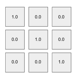
Figure 1-3. A 3 x 3 matrix
Tensors
A tensor is a multidimensional array at the most fundamental level. It is a more general mathematical structure than a vector. We can look at a vector as simply a subclass of tensors.
With tensors, the rows extend along the y-axis and the columns along the x-axis. Each axis is a dimension, and tensors have additional dimensions. Tensors also have a rank. Comparatively, a scalar is of rank 0 and a vector is rank 1. We also see that a matrix is rank 2. Any entity of rank 3 and above is considered a tensor.
Hyperplanes
Another linear algebra object you should be aware of is the hyperplane. In the field of geometry, the hyperplane is a subspace of one dimension less than its ambient space. In a three-dimensional space, the hyperplanes would have two dimensions. In two-dimensional space we consider a one-dimensional line to be a hyperplane.
A hyperplane is a mathematical construct that divides an n-dimensional space into separate “parts” and therefore is useful in applications like classification. Optimizing the parameters of the hyperplane is a core concept in linear modeling, as you’ll see further on in this chapter.
Relevant Mathematical Operations
In this section, we briefly review common linear algebra operations you should know.
Dot product
A core linear algebra operation we see often in machine learning is the dot product. The dot product is sometimes called the “scalar product” or “inner product." The dot product takes two vectors of the same length and returns a single number. This is done by matching up the entries in the two vectors, multiplying them, and then summing up the products thus obtained. Without getting too mathematical (immediately), it is important to mention that this single number encodes a lot of information.
To begin with, the dot product is a measure of how big the individual elements are in each vector. Two vectors with rather large values can give rather large results, and two vectors with rather small values can give rather small values. When the relative values of these vectors are accounted for mathematically with something called normalization, the dot product is a measure of how similar these vectors are. This mathematical notion of a dot product of two normalized vectors is called the cosine similarity.
Element-wise product
Another common linear algebra operation we see in practice is the element-wise product (or the “Hadamard product”). This operation takes two vectors of the same length and produces a vector of the same length with each corresponding element multiplied together from the two source vectors.
Converting Data Into Vectors
In the course of working in machine learning and data science we need to analyze all types of data. A key requirement is being able to take each data type and represent it as a vector. In machine learning we use many types of data (e.g., text, time-series, audio, images, and video).
So, why can’t we just feed raw data to our learning algorithm and let it handle everything? The issue is that machine learning is based on linear algebra and solving sets of equations. These equations expect floating-point numbers as input so we need a way to translate the raw data into sets of floating-point numbers. We’ll connect these concepts together in the next section on solving these sets of equations. An example of raw data would be the canonical iris dataset:
5.1,3.5,1.4,0.2,Iris-setosa
4.9,3.0,1.4,0.2,Iris-setosa
4.7,3.2,1.3,0.2,Iris-setosa
7.0,3.2,4.7,1.4,Iris-versicolor
6.4,3.2,4.5,1.5,Iris-versicolor
6.9,3.1,4.9,1.5,Iris-versicolor
5.5,2.3,4.0,1.3,Iris-versicolor
6.5,2.8,4.6,1.5,Iris-versicolor
6.3,3.3,6.0,2.5,Iris-virginica
5.8,2.7,5.1,1.9,Iris-virginica
7.1,3.0,5.9,2.1,Iris-virginica
Another example might be a raw text document:
Go, Dogs. Go!
Go on skates
or go by bike.
Both cases involve raw data of different types, yet both need some level of vectorization to be of the form we need to do machine learning. At some point, we want our input data to be in the form of a matrix but we can convert the data to intermediate representations (e.g., “svmlight” file format, shown in the code example that follows). We want our machine learning algorithm’s input data to look more like the serialized sparse vector format svmlight, as shown in the following example:
1.0 1:0.7500000000000001 2:0.41666666666666663 3:0.702127659574468 4:0.
  5652173913043479
2.0 1:0.6666666666666666 2:0.5 3:0.9148936170212765 4:0.6956521739130436
2.0 1:0.45833333333333326 2:0.3333333333333336 3:0.8085106382978723 4:0
  .7391304347826088
0.0 1:0.1666666666666665 2:1.0 3:0.021276595744680823
2.0 1:1.0 2:0.5833333333333334 3:0.9787234042553192 4:0.8260869565217392
1.0 1:0.3333333333333333 3:0.574468085106383 4:0.47826086956521746
1.0 1:0.7083333333333336 2:0.7500000000000002 3:0.6808510638297872 4:0
  .5652173913043479
1.0 1:0.916666666666667 2:0.6666666666666667 3:0.7659574468085107 4:0
  .5652173913043479
0.0 1:0.08333333333333343 2:0.5833333333333334 3:0.021276595744680823
2.0 1:0.6666666666666666 2:0.8333333333333333 3:1.0 4:1.0
1.0 1:0.9583333333333335 2:0.7500000000000002 3:0.723404255319149 4:0
  .5217391304347826
0.0 2:0.7500000000000002
This format can quickly be read into a matrix and a column vector for the labels (the first number in each row in the preceding example). The rest of the indexed numbers in the row are inserted into the proper slot in the matrix as “features” at runtime to get ready for various linear algebra operations during the machine learning process. We’ll discuss the process of vectorization in more detail in Chapter 8.
Here’s a very common question: “why do machine learning algorithms want the data represented (typically) as a (sparse) matrix?” To understand that, let’s make a quick detour into the basics of solving systems of equations.
Solving Systems of Equations
In the world of linear algebra, we are interested in solving systems of linear equations of the form:
- Ax = b
where A is a matrix of our set of input row vectors and b is the column vector of labels for each vector in the A matrix. If we take the first three rows of serialized sparse output from the previous example and place the values in its linear algebra form, it looks like this:
|
Column 1 |
Column 2 |
Column 3 |
Column 4 |
|
0.7500000000000001 |
0.41666666666666663 |
0.702127659574468 |
0.5652173913043479 |
|
0.6666666666666666 |
0.5 |
0.9148936170212765 |
0.6956521739130436 |
|
0.45833333333333326 |
0.3333333333333336 |
0.8085106382978723 |
0.7391304347826088 |
This matrix of numbers is our A variable in our equation, and each independent value or value in each row is considered a feature of our input data.
We want to find coefficients for each column in a given row for a predictor function that give us the output b, or the label for each row. The labels from the serialized sparse vectors we looked at earlier would be as follows:
|
Labels |
|
1.0 |
|
2.0 |
|
2.0 |
The coefficients mentioned earlier become the x column vector (also called the parameter vector) shown in Figure 1-4.
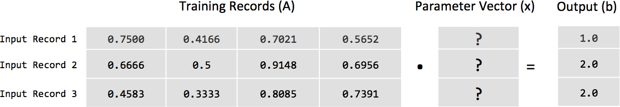
Figure 1-4. Visualizing the equation Ax = b
This system is said to be “consistent” if there exists a parameter vector x such that the solution to this equation can be directly written as follows:
It’s important to delineate the expression x = A-1b from the method of actually computing the solution. This expression only represents the solution itself. The variable A-1 is the matrix A inverted and is computed through a process called matrix inversion. Given that not all matrices can be inverted, we’d like a method to solve this equation that does not involve matrix inversion. One method is called matrix decomposition. An example of matrix decomposition in solving systems of linear equations is using lower upper (LU) decomposition to solve for the matrix A. Beyond matrix decomposition, let’s take a look at the general methods for solving sets of linear equations.
Methods for solving systems of linear equations
There are two general methods for solving a system of linear equations. The first is called the “direct method,” in which we know algorithmically that there are a fixed number of computations. The other approach is a class of methods known as iterative methods, in which through a series of approximations and a set of termination conditions we can derive the parameter vector x. The direct class of methods is particularly effective when we can fit all of the training data (A and b) in memory on a single computer. Well-known examples of the direct method of solving sets of linear equations are Gaussian Elimination and the Normal Equations.
Iterative methods
The iterative class of methods is particularly effective when our data doesn’t fit into the main memory on a single computer, and looping through individual records from disk allows us to model a much larger amount of data. The canonical example of iterative methods most commonly seen in machine learning today is Stochastic Gradient Descent (SGD), which we discuss later in this chapter. Other techniques in this space are Conjugate Gradient Methods and Alternating Least Squares (discussed further in Chapter 3). Iterative methods also have been shown to be effective in scale-out methods, for which we not only loop through local records, but the entire dataset is sharded across a cluster of machines, and periodically the parameter vector is averaged across all agents and then updated at each local modeling agent (described in more detail in Chapter 9).
Iterative methods and linear algebra
At the mathematical level, we want to be able to operate on our input dataset with these algorithms. This constraint requires us to convert our raw input data into the input matrix A. This quick overview of linear algebra gives us the “why” for going through the trouble to vectorize data. Throughout this book, we show code examples of converting the raw input data into the input matrix A, giving you the “how.” The mechanics of how we vectorize our data also affects the results of the learning process. As we’ll see later in the book, how we handle data in the preprocess stage before vectorization can create more accurate models.
The Math Behind Machine Learning: Statistics
Let’s review just enough statistics to let this chapter move forward. We need to highlight some basic concepts in statistics, such as the following:
- Probabilities
- Distributions
- Likelihood
There are also some other basic relationships we’d like to highlight in descriptive statistics and inferential statistics. Descriptive statistics include the following:
- Histograms
- Boxplots
- Scatterplots
- Mean
- Standard deviation
- Correlation coefficient
This contrasts with how inferential statistics are concerned with techniques for generalizing from a sample to a population. Here are some examples of inferential statistics:
- p-values
- credibility intervals
The relationship between probability and inferential statistics:
- Probability reasons from the population to the sample (deductive reasoning)
- Inferential statistics reason from the sample to the population
Before we can understand what a specific sample tells us about the source population, we need to understand the uncertainty associated with taking a sample from a given population.
Regarding general statistics, we won’t linger on what is an inherently broad topic already covered in depth by other books. This section is in no way meant to serve as a true statistics review; rather, it is designed to direct you toward relevant topics that you can investigate in greater depth from other resources. With that disclaimer out of the way, let’s begin by defining probability in statistics.
Probability
We define probability of an event E as a number always between 0 and 1. In this context, the value 0 infers that the event E has no chance of occurring, and the value 1 means that the event E is certain to occur. Many times we’ll see this probability expressed as a floating-point number, but we also can express it as a percentage between 0 and 100 percent; we will not see valid probabilities lower than 0 percent and greater than 100 percent. An example would be a probability of 0.35 expressed as 35 percent (e.g., 0.35 x 100 == 35 percent).
The canonical example of measuring probability is observing how many times a fair coin flipped comes up heads or tails (e.g., 0.5 for each side). The probability of the sample space is always 1 because the sample space represents all possible outcomes for a given trial. As we can see with the two outcomes (“heads” and its complement, “tails”) for the flipped coin, 0.5 + 0.5 == 1.0 because the total probability of the sample space must always add up to 1. We express the probability of an event as follows:
- P( E ) = 0.5
And we read this like so:
The probability of an event E is 0.5
Probability is at the center of neural networks and deep learning because of its role in feature extraction and classification, two of the main functions of deep neural networks. For a larger review of statistics, check out O’Reilly’s Statistics in a Nutshell: A Desktop Quick Reference by Boslaugh and Watters.
Conditional Probabilities
When we want to know the probability of a given event based on the existing presence of another event occurring, we express this as a conditional probability. This is expressed in literature in the form:
- P( E | F )
where:
E is the event for which we’re interested in a probability.
F is the event that has already occurred.
An example would be expressing how a person with a healthy heart rate has a lower probability of ICU death during a hospital visit:
P(ICU Death | Poor Heart Rate) > P(ICU Death | Healthy Heart Rate)
Sometimes, we’ll hear the second event, F, referred to as the “condition.” Conditional probability is interesting in machine learning and deep learning because we’re often interested in when multiple things are happening and how they interact. We’re interested in conditional probabilities in machine learning in the context in which we’d learn a classifier by learning
- P ( E | F )
where E is our label and F is a number of attributes about the entity for which we’re predicting E. An example would be predicting mortality (here, E) given that measurements taken in the ICU for each patient (here, F).
Posterior Probability
In Bayesian statistics, we call the posterior probability of the random event the conditional probability we assign after the evidence is considered. Posterior probability distribution is defined as the probability distribution of an unknown quantity conditional on the evidence collected from an experiment treated as a random variable. We see this concept in action with softmax activation functions (explained later in this chapter), in which raw input values are converted to posterior probabilities.
Distributions
A probability distribution is a specification of the stochastic structure of random variables. In statistics, we rely on making assumptions about how the data is distributed to make inferences about the data. We want a formula that specifies how frequent values of observations in the distribution are and how values can be taken by points in the distribution. A common distribution is known as the normal distribution (also called Gaussian distribution, or the bell curve). We like to fit a dataset to a distribution because if the dataset is reasonably close to the distribution, we can make assumptions based on the theoretical distribution in how we operate with the data.
We classify distributions as continuous or discrete. A discrete distribution has data that can assume only certain values. In a continuous distribution, data can be any value within the range. An example of a continuous distribution would be normal distribution. An example of a discrete distribution would be binomial distribution.
Normal distribution allows us to assume sampling distributions of statistics (e.g., “sample mean”) are normally distributed under specified conditions. The normal distribution (see Figure 1-5), or Gaussian distribution, was named after the eighteenth-century mathematician and physicist Karl Gauss. Normal distribution is defined by its mean and standard deviation and has generally the same shape across all variations.
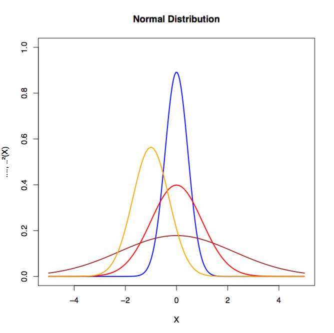
Figure 1-5. Examples of normal distributions
Other relevant distributions in machine learning include the following:
- Binomial distribution
- Inverse Gaussian distribution
- Log normal distribution
Distribution of the training data in machine learning is important to understand how to vectorize the data for modeling.
A long-tailed distribution (such as Zipf, power laws, and Pareto distributions) is a scenario in which a high-frequency population is followed by a low-frequency population that gradually decreases in asymptotic fashion. These distributions were discovered by Benoit Mandelbrot in the 1950s and later popularized by the writer Chris Anderson in his book The Long Tail: Why the Future of Business is Selling Less of More.
An example would be ranking the items a retailer sells among which a few items are exceptionally popular and then we see a large number of unique items with relatively small quantities sold. This rank-frequency distribution (primarily of popularity or “how many were sold”) often forms power laws. From this perspective, we can consider them to be long-tailed distributions.
We see these long-tailed distributions manifested in the following:
- Earthquake damage
-
The damage becomes worse as the scale of the quake increases, so worse case shifts.
- Crop yields
-
We sometimes see events outside of the historical record, whereas our model tends to be tuned around the mean.
- Predicting fatality post ICU visit
-
We can have events far outside the scope of what happens inside the ICU visit that affect mortality.
These examples are relevant in the context of this book for classification problems because most statistical models depend on inference from lots of data. If the more interesting events occur out in the tail of the distribution and we don’t have this represented in the training sample data, our model might perform unpredictably. This effect can be enhanced in nonlinear models such as neural networks. We’d consider this situation the special case of the “in sample/out of sample” problem. Even a seasoned machine learning practitioner can be surprised at how well a model performs on a skewed training data sample yet fails to generalize well on the larger population of data.
Long-tailed distributions deal with the real possibility of events occurring that are five times the standard deviation. We must be mindful to get a decent representation of events in our training data to prevent overfitting the training data. We’ll look in greater detail at ways to do this later when we talk about overfitting and then in Chapter 4 on tuning.
Samples Versus Population
A population of data is defined as all of the units we’d like to study or model in our experiment. An example would be defining our population of study as “all Java programmers in the state of Tennessee.”
A sample of data is a subset of the population of data that hopefully represents the accurate distribution of the data without introducing sampling bias (e.g., skewing the sample distribution based on how we sampled the population).
Resampling Methods
Bootstrapping and cross-validation are two common methods of resampling in statistics that are useful to machine learning practitioners. In the context of machine learning with bootstrapping, we’re drawing random samples from another sample to generate a new sample that has a balance between the number of samples per class. This is useful when we’d like to model against a dataset with highly unbalanced classes.
Cross-validation (also called rotation estimation) is a method to estimate how well a model generalizes on a training dataset. In cross-validation we split the training dataset into N number of splits and then separate the splits into training and test groups. We train on the training group of splits and then test the model on the test group of splits. We rotate the splits between the two groups many times until we’ve exhausted all the variations. There is no hard number for the number of splits to use but researchers have found 10 splits to work well in practice. It also is common to see a separate portion of the held-out data used as a validation dataset during training.
Selection Bias
In selection bias we’re dealing with a sampling method that does not have proper randomization and skews the sample in a way such that the sample is not representative of the population we’d like to model. We need to be aware of selection bias when resampling datasets so that we don’t introduce bias into our models that will lower our model’s accuracy on data from the larger population.
Likelihood
When we discuss the likeliness that an event will occur yet do not specifically reference its numeric probability, we’re using the informal term, likelihood. Typically, when we use this term, we’re talking about an event that has a reasonable probability of happening but still might not. There also might be factors not yet observed that will influence the event, as well. Informally, likelihood is also used as a synonym for probability.
How Does Machine Learning Work?
In a previous section on solving systems of linear equations, we introduced the basics of solving Ax = b. Fundamentally, machine learning is based on algorithmic techniques to minimize the error in this equation through optimization.
In optimization, we are focused on changing the numbers in the x column vector (parameter vector) until we find a good set of values that gives us the closest outcomes to the actual values. Each weight in the weight matrix will be adjusted after the loss function calculates the error (based on the actual outcome, as shown earlier, as the b column vector) produced by the network. An error matrix attributing some portion of the loss to each weight will be multiplied by the weights themselves.
We discuss SGD further on in this chapter as one of the major methods to perform machine learning optimization, and then we’ll connect these concepts to other optimization algorithms as the book progresses. We’ll also cover the basics of hyperparameters such as regularization and learning rate.
Regression
Regression refers to functions that attempt to predict a real value output. This type of function estimates the dependent variable by knowing the independent variable. The most common class of regression is linear regression, based on the concepts we’ve previously described in modeling systems of linear equations. Linear regression attempts to come up with a function that describes the relationship between x and y, and, for known values of x, predicts values of y that turn out to be accurate.
Setting up the model
The prediction of a linear regression model is the linear combination of coefficients (from the parameter vector x) and then input variables (features from the input vector). We can model this by using the following equation:
- y = a + Bx
where a is the y-intercept, B is the input features, and x is the parameter vector.
This equation expands to the following:
A simple example of a problem that linear regression solves would be predicting how much we’d spend per month on gasoline based on the length of our commute. Here, what you pay at the tank is a function of how far you drive. The gas cost is the dependent variable and the length of the commute is the independent variable. It’s reasonable to keep track of these two quantities and then define a function, like so:
- cost = f (distance)
This allows us to reasonably predict our gasoline spending based on mileage. In this example, we’d consider distance to be our independent variable and cost to be the dependent variable in our model f.
Here are some other examples of linear regression modeling:
- Predicting weight as a function of height
- Predicting a house’s sale price based on its square footage
Visualizing linear regression
Visually, we can represent linear regression as finding a line that comes as close to as many points as possible in a scatterplot of data, as demonstrated in Figure 1-6.
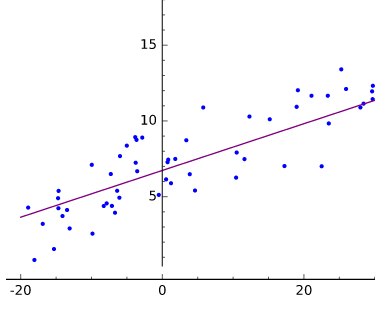
Figure 1-6. Linear regression plotted
Fitting is defining a function f(x) that produces y-values close to the measured or real-world y values. The line produced by y = f(x) comes close to the scattered coordinates, the pairs of dependent and independent variables.
Relating the linear regression model
We can relate this function to the earlier equation, Ax = b, where A is the features (e.g., “weight” or “square footage”) for all of the input examples that we want to model. Each input record is a row in the matrix A. The column vector b is the outcomes for all of the input records in the A matrix. Using an error function and an optimization method (e.g., SGD), we can find a set of x parameters such that we minimize the error across all of the predictions versus the true outcomes.
Using SGD, as we discussed earlier, we’d have three components to solve for our parameter vector x:
- A hypothesis about the data
-
The inner product of the parameter vector x and the input features (as displayed above)
- A cost function
-
Squared error (prediction – actual) of prediction
- An update function
-
The derivative of the squared error loss function (cost function)
While linear regression deals with straight lines, nonlinear curve fitting handles everything else, most notably curves that deal with x to higher exponents than 1. (That’s why we hear machine learning sometimes described as “curve fitting.”) An absolute fit would hit every dot on a scatterplot. Ironically, absolute fit is usually a very poor outcome, because it means your model has trained too perfectly on the training set, and has almost no predictive power beyond the data it has seen (e.g., does not generalize well), as we previously discussed.
Classification
Classification is modeling based on delineating classes of output based on some set of input features. If regression give us an outcome of "how much,” classification gives us an outcome of "what kind.” The dependent variable y is categorical rather than numerical.
The most basic form of classification is a binary classifier that only has a single output with two labels (two classes: 0 and 1, respectively). The output can also be a floating-point number between 0.0 and 1.0 to indicate a classification below absolute certainty. In this case, we need to determine a threshold (typically 0.5) at which we delineate between the two classes. These classes are often referred to as positive classification in the literature (e.g., 1.0) and then negative (e.g., 0.0) classifications. We’ll talk more about this in “Evaluating Models”.
Examples of binary classification include:
- Classifying whether someone has a disease or not
- Classifying an email as spam or not spam
- Classifying a transaction as fraudulent or nominal
Beyond two labels, we can have classification models that have N labels for which we’d score each of the output labels, and then the label with the highest score is the output label. We’ll discuss this further as we talk about neural networks with multiple outputs versus neural networks with a single output (binary classification). We’ll also discuss classification more in this chapter when we talk about logistic regression and then dive into the full architecture of neural networks.
Clustering
Clustering is an unsupervised learning technique that involves using a distance measure and iteratively moving similar items more closely together. At the end of the process, the items clustered most densely around n centroids are considered to be classified in that group. K-means clustering is one of the more famous variations of clustering in machine learning.
Underfitting and Overfitting
As we mentioned earlier, optimization algorithms first attempt to solve the problem of underfitting; that is, of taking a line that does not approximate the data well and making it approximate the data better. A straight line cutting across a curving scatterplot would be a good example of underfitting, as is illustrated in Figure 1-7.
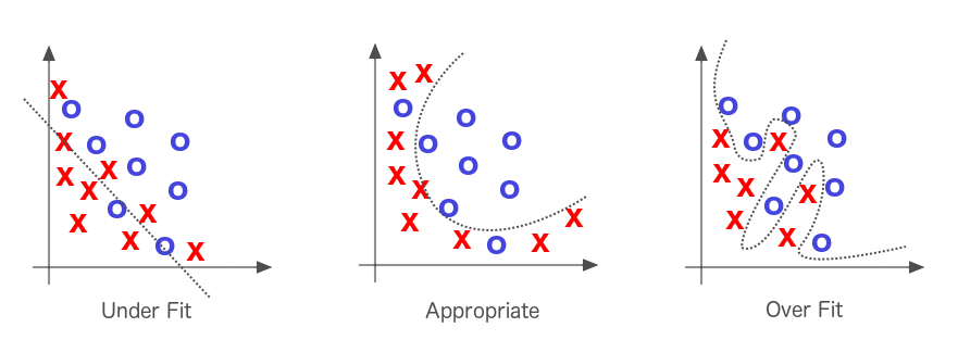
Figure 1-7. Underfitting and overfitting in machine learning
If the line fits the data too well, we have the opposite problem, called “overfitting.” Solving underfitting is the priority, but much effort in machine learning is spent attempting not to overfit the line to the data. When we say a model overfits a dataset, we mean that it may have a low error rate for the training data, but it does not generalize well to the overall population of data in which we’re interested.
Another way of explaining overfitting is by thinking about probable distributions of data. The training set of data that we’re trying to draw a line through is just a sample of a larger unknown set, and the line we draw will need to fit the larger set equally well if it is to have any predictive power. We must assume, therefore, that our sample is loosely representative of a larger set.
Optimization
The aforementioned process of adjusting weights to produce more and more accurate guesses about the data is known as parameter optimization. You can think of this process as a scientific method. You formulate a hypothesis, test it against reality, and refine or replace that hypothesis again and again to better describe events in the world.
Every set of weights represents a specific hypothesis about what inputs mean; that is, how they relate to the meanings contained in one’s labels. The weights represent conjectures about the correlations between networks’ input and the target labels they seek to guess. All possible weights and their combinations can be described as the hypothesis space of this problem. Our attempt to formulate the best hypothesis is a matter of searching through that hypothesis space, and we do so by using error and optimization algorithms. The more input parameters we have, the larger the search space of our problem. Much of the work of learning is deciding which parameters to ignore and which to hear.
The Decision Boundary and Hyperplanes
When we mention the “decision boundary,” we’re talking about the n-dimensional hyperplane created by the parameter vector in linear modeling.
Fitting lines to data by gauging their cost (i.e., their distance from the ground-truth data points) is at the center of machine learning. The line should more or less fit the data, and it does so by minimizing the aggregate distance of all points from the line. You minimize the sum of the difference between the line at point x and the target point y to which it corresponds. In a three-dimensional space, you can imagine the error-scape of hills and valleys, and picture your algorithm as a blind hiker who feels for the slope. An optimization algorithm, like gradient descent, is what informs the hiker which direction is downhill so that she knows where to step.
The goal is to find the weights that minimize the difference between what your network predicts (, or the dot-product of A and x) and what your test set knows to be true (b), as we saw earlier in Figure 1-4. The parameter vector (x) above is where you would find the weights. The accuracy of a network is a function of its input and parameters, and the speed at which it becomes accurate is a function of its hyperparameters.
Hyperparameters
In machine learning, we have both model parameters and then we have parameters we tune to make networks train better and faster. These tuning parameters are called hyperparameters, and they deal with controlling optimization function and model selection during training with our learning algorithm.
Convergence
Convergence refers to an optimization algorithm finding values for a parameter vector that gives our optimization algorithm the smallest error possible across all training examples. The optimization algorithm is said to “converge” on the solution iteratively after it tries several different variations of the parameters.
Following are the three important functions at work in machine learning optimization:
- Parameters
-
Transform input to help determine the classifications a network infers
- Loss function
-
Gauges how well it classifies (minimizes error) at each step
- Optimization function
-
Guides it toward the points of least error
Now, let’s take a closer look at one subclass of optimization called convex optimization.
Convex Optimization
In convex optimization, learning algorithms deal with convex cost functions. If the x-axis represents a single weight, and the y-axis represents that cost, the cost will descend as low as 0 at one point on the x-axis and rise exponentially on either side as the weight strays away from its ideal in two directions.
Figure 1-8 demonstrates that we also can turn the idea of a cost function upside down.
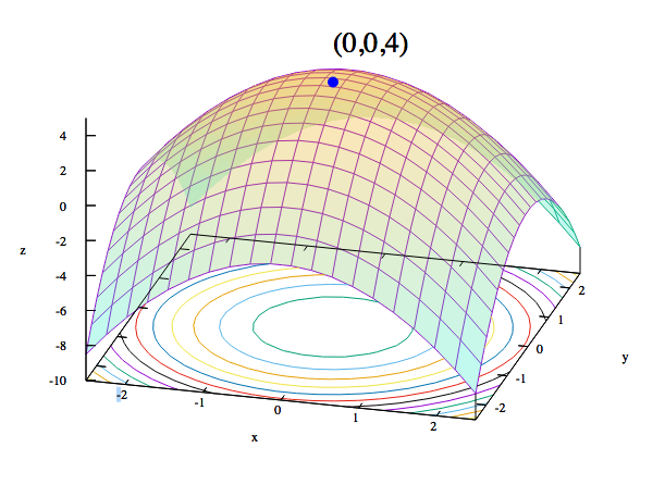
Figure 1-8. Visualizing convex functions
Another way to relate parameters to the data is with a maximum likelihood estimation, or MLE. The MLE traces a parabola whose edges point downward, with likelihood measured on the vertical axis, and a parameter on the horizontal. Each point on the parabola measures the likelihood of the data, given a certain set of parameters. The goal of MLE is to iterate over possible parameters until it finds the set that makes the given data most likely.
In a sense, maximum likelihood and minimum cost are two sides of the same coin. Calculating the cost function of two weights against the error (which puts us in a three-dimensional space) will produce something that looks more like a sheet held at each corner and drooping convexly in the middle—a rather bowl-shaped function. The slopes of these convex curves allow our algorithm a hint as to what direction to take the next parameter step, as we’ll see in the gradient descent optimization algorithm discussed next.
Gradient Descent
In gradient descent, we can imagine the quality of our network’s predictions (as a function of the weight/parameter values) as a landscape. The hills represent locations (parameter values or weights) that give a lot of prediction error; valleys represent locations with less error. We choose one point on that landscape at which to place our initial weight. We then can select the initial weight based on domain knowledge (if we’re training a network to classify a flower species we know petal length is important, but color isn’t). Or, if we’re letting the network do all the work, we might choose the initial weights randomly.
The purpose is to move that weight downhill, to areas of lower error, as quickly as possible. An optimization algorithm like gradient descent can sense the actual slope of the hills with regard to each weight; that is, it knows which direction is down. Gradient descent measures the slope (the change in error caused by a change in the weight) and takes the weight one step toward the bottom of the valley. It does so by taking a derivative of the loss function to produce the gradient. The gradient gives the algorithm the direction for the next step in the optimization algorithm, as depicted in Figure 1-9.
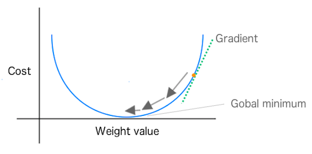
Figure 1-9. Showing weight changes toward global minimum in SGD
The derivative measures “rate of change” of a function. In convex optimization, we’re looking for the point at which the derivative is equal to 0 for the function. This point is also known as the stationary point of the function or the minimum point. In optimization, we consider optimizing a function to be minimizing a function (outside of inverting the cost function).
This process of measuring loss and changing the weight by one step in the direction of less error is repeated until the weight arrives at a point beyond which it cannot go lower. It stops in the trough, the point of greatest accuracy. When using a convex loss function (typically in linear modeling), we see a loss function that has only a global minimum.
You can think of linear modeling in terms of three components to solve for our parameter vector x:
- A hypothesis about the data; for example, “the equation we use to make a prediction in the model.”
- A cost function. Also called a loss function; for example, “sum of squared errors.”
- An update function; we take the derivative of the loss function.
Our hypothesis is the combination of the learned parameters x and the input values (features) that gives us a classification or real valued (regression) output. The cost function tells us how far we are from the global minimum of the loss function, and we use the derivative of the loss function as the update function to change the parameter vector x.
Taking the derivative of the loss function indicates for each parameter in x the degree to which we need to adjust the parameter to get closer to the 0-point on the loss curves. We’ll look more closely at these equations later on in this chapter when we show how they work for both linear regression and logistic regression (classification).
However, in other nonlinear problems we don’t always get such a clean loss curve. The problem with these other nonlinear hypothetical landscapes is that there might be several valleys, and gradient descent’s mechanism for taking the weight lower cannot know if it has reached the lowest valley or simply the lowest point in a higher valley, so to speak. The lowest point in the lowest valley is known as the global minimum, whereas the nadirs of all other valleys are known as local minima. If gradient descent reaches a local minimum, it is effectively trapped, and this is one drawback of the algorithm. We’ll look at ways to overcome this issue in Chapter 6 when we examine hyperparameters and learning rate.
A second problem that gradient descent encounters is with non-normalized features. When we write “non-normalized features,” we mean features that can be measured by very different scales. If you have one dimension measured in the millions, and another in decimals, gradient descent will have a difficult time finding the steepest slope to minimize error.
Dealing with Normalization
In Chapter 8 we take an extended look at methods of normalization in the context of vectorization and illustrate some ways to better deal with this issue.
Stochastic Gradient Descent
In gradient descent we’d calculate the overall loss across all of the training examples before calculating the gradient and updating the parameter vector. In SGD, we compute the gradient and parameter vector update after every training sample. This has been shown to speed up learning and also parallelizes well as we’ll talk about more later in the book. SGD is an approximation of “full batch” gradient descent.
Mini-batch training and SGD
Another variant of SGD is to use more than a single training example to compute the gradient but less than the full training dataset. This variant is referred to as the mini-batch size of training with SGD and has been shown to be more performant than using only single training instances. Applying mini-batch to stochastic gradient descent has also shown to lead to smoother convergence because the gradient is computed at each step it uses more training examples to compute the gradient.
As the mini-batch size increases the gradient computed is closer to the “true” gradient of the entire training set. This also gives us the advantage of better computational efficiency. If our mini-batch size is too small (e.g., 1 training record), we’re not using hardware as effectively as we could, especially for situations such as GPUs. Conversely, making the mini-batch size larger (beyond a point) can be inefficient, as well, because we can produce the same gradient with less computational effort (in some cases) with regular gradient descent.
Quasi-Newton Optimization Methods
Quasi-Newton optimization methods are iterative algorithms that involve a series of “line searches.” Their distinguishing feature with respect to other optimization methods is how they choose the search direction. These methods are discussed further in later chapters of the book.
Generative Versus Discriminative Models
We can generate different types of output from a model depending on what type of model we set up. The two major types are generative models and discriminative models. Generative models understand how the data was created in order to generate a type of response or output. Discriminative models are not concerned with how the data was created and simply give us a classification or category for a given input signal. Discriminative models focus on closely modeling the boundary between classes and can yield a more nuanced representation of this boundary than a generative model. Discriminative models are typically used for classification in machine learning.
A generative model learns the joint probability distribution p(x, y), whereas a discriminative model learns the conditional probability distribution p(y|x). The distribution p(y|x) is the natural distribution for taking input x and producing an output (or classification) y, hence the name “discriminative model.” With generative models learning the distribution p(x,y), we see them used to generate likely output, given a certain input. Generative models are typically set up as probabilistic graphical models which capture the subtle relations in the data.
Logistic Regression
Logistic regression is a well-known type of classification in linear modeling. It works for both binary classification as well as for multiple labels in the form of multinomial logistic regression. Logistic regression is a regression model (technically) in which the dependent variable is categorical (e.g., “classification”). The binary logistic model is used to estimate the probability of a binary response based on a set of one or more input variables (independent variables or “features”). This output is the statistical probability of a category, given certain input predictors.
Similar to linear regression, we can express a logistic regression modeling problem in the form of Ax = b, where A is the feature (e.g., “weight” or “square footage”) for all of the input examples we want to model. Each input record is a row in the matrix A, and the column vector b is the outcomes for all of the input records in the A matrix. Using a cost function and an optimization method, we can find a set of x parameters such that we minimize the error across all of the predictions versus the true outcomes.
Again, we’ll use SGD to set up this optimization problem and we have three components to solve for our parameter vector x:
- A hypothesis about the data
- A cost function
-
“max likelihood estimation”
- An update function
-
A derivative of the cost function
In this case, the input comprises independent variables (e.g., the input columns or “features”), whereas the output is the dependent variables (e.g., “label scores”). An easy way to think about it is logistic regression function pairs input values with weights to determine whether an outcome is likely. Let’s take a closer look at the logistic function.
The Logistic Function
In logistic regression we define the logistic function (“hypothesis”) as follows:
This function is useful in logistic regression because it takes any input in the range of negative to positive infinity and maps it to output in the range of 0.0 to 1.0. This allows us to interpret the output value as a probability. Figure 1-10 shows a plot of the logistic function equation.
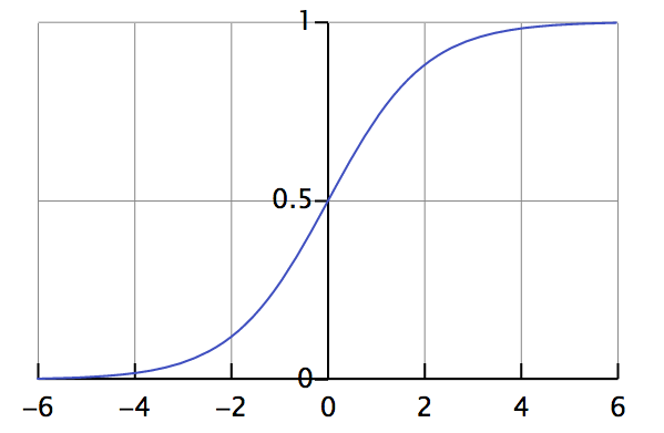
Figure 1-10. Plot of the logistic function
This function is known as a continuous log-sigmoid function with a range of 0.0 to 1.0. We’ll see this function covered again later in “Activation Functions”.
Understanding Logistic Regression Output
The logistic function is often denoted with the Greek letter sigma, or σ, because the relationship between x and y on a two-dimensional graph resembles an elongated, wind-blown “s” whose maximum and minimum asymptotically approach 1 and 0, respectively.
If y is a function of x, and that function is sigmoidal or logistic, the more x increases, the closer we come to 1/1, because e to the power of an infinitely large negative number approaches zero; in contrast, the more x decreases below zero, the more the expression (1 + e–θx) grows, shrinking the entire quotient. Because (1 + e–θx) is in the denominator, the larger it becomes, the closer the quotient itself comes to zero.
With logistic regression, f(x) represents the probability that y equals 1 (i.e., is true) given each input x. If we are attempting to estimate the probability that an email is spam, and f(x) happens to equal 0.6, we could paraphrase that by saying y has a 60 percent of being 1, or the email has a 60 percent chance of being spam, given the input. If we define machine learning as a method to infer unknown outputs from known inputs, the parameter vector x in a logistic regression model determines the strength and certainty of our deductions.
The Logit Transformation
The logit function is the inverse of the logistic function (“logistic transform”).
Evaluating Models
Evaluating models is the process of understanding how well they give the correct classification and then measuring the value of the prediction in a certain context. Sometimes, we only care how often a model gets any prediction correct; other times, it’s important that the model gets a certain type of prediction correct more often than the others. In this section, we cover topics like bad positives, harmless negatives, unbalanced classes, and unequal costs for predictions. Let’s take a look at the basic tool for evaluating models: the confusion matrix.
The Confusion Matrix
The confusion matrix (see Figure 1-11)—also called a table of confusion—is a table of rows and columns that represents the predictions and the actual outcomes (labels) for a classifier. We use this table to better understand how well the model or classifier is performing based on giving the correct answer at the appropriate time.
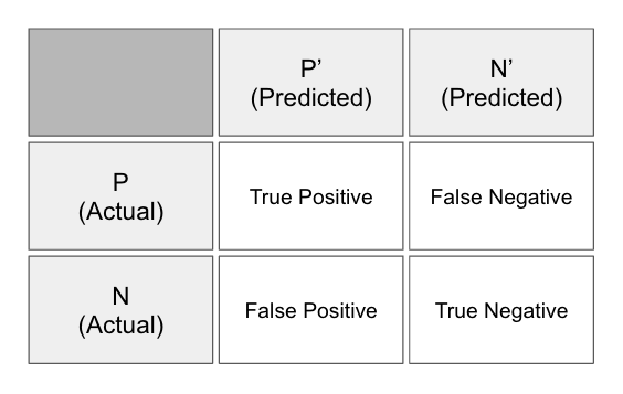
Figure 1-11. The confusion matrix
We measure these answers by counting the number of the following:
- True positives
- Positive prediction
- Label was positive
- False positives
- Positive prediction
- Label was negative
- True negatives
- Negative prediction
- Label was negative
- False negatives
- Negative prediction
- Label was positive
In traditional statistics a false positive is also known as “type I error” and a false negative is known as a “type II error.” By tracking these metrics, we can achieve a more detailed analysis on the performance of the model beyond the basic percentage of guesses that were correct. We can calculate different evaluations of the model based on combinations of the aforementioned four counts in the confusion matrix, as shown here:
 Accuracy:  0.94
 Precision: 0.8662
 Recall:    0.8955
 F1 Score:  0.8806
In the preceding example, we can see four different common measures in the evaluation of machine learning models. We’ll cover each of them shortly, but for now, let’s begin with the basics of evaluating model sensitivity versus model specificity.
Sensitivity versus specificity
Sensitivity and specificity are two different measures of a binary classification model. The true positive rate measures how often we classify an input record as the positive class and its the correct classification. This also is called sensitivity, or recall; an example would be classifying a patient as having a condition who was actually sick. Sensitivity quantifies how well the model avoids false negatives.
- Sensitivity = TP / (TP + FN)
If our model was to classify a patient from the previous example as not having the condition and she actually did not have the condition then this would be considered a true negative (also called specificity). Specificity quantifies how well the model avoids false positives.
- Specificity = TN / (TN + FP)
Many times we need to evaluate the trade-off between sensitivity and specificity. An example would be to have a model that detects serious illness in patients more frequently because of the high cost of misdiagnosing a truly sick patient. We’d consider this model to have low specificity. A serious sickness could be a danger to the patient’s life and to the others around him, so our model would be considered to have a high sensitivity to this situation and its implications. In a perfect world, our model would be 100 percent sensitive (i.e., all sick are detected) and 100 percent specific (i.e., no one who is not sick is classified as sick).
Accuracy
Accuracy is the degree of closeness of measurements of a quantity to that quantity’s true value.
- Accuracy = (TP + TN) / (TP + FP + FN + TN)
Accuracy can be misleading in the quality of the model when the class imbalance is high. If we simply classify everything as the larger class, our model will automatically get a large number of its guesses correct and provide us with a high accuracy score yet misleading indication of value based on a real application of the model (e.g., it will never predict the smaller class or rare event).
Precision
The degree to which repeated measurements under the same conditions give us the same results is called precision in the context of science and statistics. Precision is also known as the positive prediction value. Although sometimes used interchangeably with “accuracy” in colloquial use, the terms are defined differently in the frame of the scientific method.
- Precision = TP / (TP + FP)
A measurement can be accurate yet not precise, not accurate but still precise, neither accurate nor precise, or both accurate and precise. We consider a measurement to be valid if it is both accurate and precise.
F1
In binary classification we consider the F1 score (or F-score, F-measure) to be a measure of a model’s accuracy. The F1 score is the harmonic mean of both the precision and recall measures (described previously) into a single score, as defined here:
- F1 = 2TP / (2TP + FP + FN)
We see scores for F1 between 0.0 and 1.0, where 0.0 is the worst score and 1.0 is the best score we’d like to see. The F1 score is typically used in information retrieval to see how well a model retrieves relevant results. In machine learning, we see the F1 score used as an overall score on how well our model is performing.
Context and interpreting scores
Context can play a role in how we evaluate our model and dictate when we use different types of scores, as described previously in this section. Class imbalance can play a large role in dictating choice of evaluation score, and in many datasets, we’ll find that the classes or label counts are not well balanced. Here are some typical domains in which we see this:
- Web click prediction
- ICU mortality prediction
- Fraud detection
In these contexts, an overall “percent correct” score can be misleading to the overall value, in practical terms, of the model. An example of this would be the PhysioNet Challenge dataset from 2012.
The goal of the challenge was to “predict in-hospital mortality with the greatest accuracy using a binary classifier.” The difficulty and challenge in modeling this dataset is that predicting that a patient will live is the easy part because the bulk of examples in the dataset have outcomes in which the patient does live. Predicting death accurately in this scenario is the goal; this is where the model has the most value in the context of being clinically relevant in the real world. In this competition, the scores were calculate as follows:
- Score = MIN(Precision, Recall)
This was set up such that it kept the contestants focused on not just predicting that the patient would live most of the time and get a nice F1 score, but focus on predicting when the patient would die (keeping the focus on being clinically relevant). This is a great example of how context can change how we evaluate our models.
Methods to Handle Class Imbalance
In Chapter 6 we illustrate practical ways to deal with class imbalance. We take a closer look at the different facets of class imbalance and error distributions in the context of classification and regression.
Building an Understanding of Machine Learning
In this chapter, we introduced the core concepts needed for practicing machine learning. We looked at the core mathematical concepts of modeling based around the equation:
- Ax = b
We also looked at the core ideas of getting features into the matrix A, ways to change the parameter vector x, and setting the outcomes in the vector b. We illustrated some basic ways to change the parameter vector x to minimize the score (or “loss”) of the objective function.
As we move forward in this book, we’ll continue to expand on these key concepts. We’ll see how neural networks and deep learning are based on these fundamentals but add more complex ways to create the A matrix, change the x parameter vector through optimization methods, and measure loss during training. Let’s now move on to Chapter 2, where we build further on these concepts with the basics of neural networks.
1 Patterson. 2008. “TinyTermite: A Secure Routing Algorithm” and Sartipi and Patterson. 2009. “TinyTermite: A Secure Routing Algorithm on Intel Mote 2 Sensor Network Platform.”
2 Gatys et. al, 2015. “A Neural Algorithm of Artistic Style.”
Get Deep Learning now with the O’Reilly learning platform.
O’Reilly members experience books, live events, courses curated by job role, and more from O’Reilly and nearly 200 top publishers.

