Chapter 4. In-Memory Computing with Spark
Together, HDFS and MapReduce have been the foundation of and the driver for the advent of large-scale machine learning, scaling analytics, and big data appliances for the last decade. Like most platform technologies, the maturation of Hadoop has led to a stable computing environment that is general enough to build specialist tools for tasks such as graph processing, micro-batch processing, SQL querying, data warehousing, and machine learning. However, as Hadoop became more widely adopted, more specializations were required for a wider variety of new use cases, and it became clear that the batch processing model of MapReduce was not well suited to common workflows including iterative, interactive, or on-demand computations upon a single dataset.
The primary MapReduce abstraction (specification of computation as a mapping then a reduction) is parallelizable, easy to understand, and hides the details of distributed computing, thus allowing Hadoop to guarantee correctness. However, in order to achieve coordination and fault tolerance, the MapReduce model uses a pull execution model that requires intermediate writes of data back to HDFS. Unfortunately, the input/output (I/O) of moving data from where it’s stored to where it needs to be computed upon is the largest time cost in any computing system; as a result, while MapReduce is incredibly safe and resilient, it is also necessarily slow on a per-task basis. Worse, almost all applications must chain multiple MapReduce jobs together in multiple steps, creating a data flow toward the final required result. This results in huge amounts of intermediate data written to HDFS that is not required by the user, creating additional costs in terms of disk usage.
To address these problems, Hadoop has moved to a more general resource management framework for computation: YARN. Whereas previously the MapReduce application allocated resources (processors, memory) to jobs specifically for mappers and reducers, YARN provides more general resource access to Hadoop applications. The result is that specialized tools no longer have to be decomposed into a series of MapReduce jobs and can become more complex. By generalizing the management of the cluster, the programming model first imagined in MapReduce can be expanded to include new abstractions and operations.
Spark is the first fast, general-purpose distributed computing paradigm resulting from this shift, and is rapidly gaining popularity particularly because of its speed and adaptability. Spark primarily achieves this speed via a new data model called resilient distributed datasets (RDDs) that are stored in memory while being computed upon, thus eliminating expensive intermediate disk writes. It also takes advantage of a directed acyclic graph (DAG) execution engine that can optimize computation, particularly iterative computation, which is essential for data theoretic tasks such as optimization and machine learning. These speed gains allow Spark to be accessed in an interactive fashion (as though you were sitting at the Python interpreter), making the user an integral part of computation and allowing for data exploration of big datasets that was not previously possible, bringing the cluster to the data scientist.
Note
Because directed acyclic graphs are commonly used to describe the steps in a data flow, the term DAG is used often when discussing big data processing. In this sense, DAGs are directed because one step or steps follow after another, and acylic because a single step does not repeat itself. When a data flow is described as a DAG, it eliminates costly synchronization and makes parallel applications easier to build.
In this chapter, we introduce Spark and resilient distributed datasets. This is the last chapter describing the nuts and bolts of doing analytics with Hadoop. Because Spark implements many applications already familiar to data scientists (e.g., DataFrames, interactive notebooks, and SQL), we propose that at least initially, Spark will be the primary method of cluster interaction for the novice Hadoop user. To that end, we describe RDDs, explore the use of Spark on the command line with pyspark, then demonstrate how to write Spark applications in Python and submit them to the cluster as Spark jobs.
Spark Basics
Apache Spark is a cluster-computing platform that provides an API for distributed programming similar to the MapReduce model, but is designed to be fast for interactive queries and iterative algorithms.1 It primarily achieves this by caching data required for computation in the memory of the nodes in the cluster. In-memory cluster computation enables Spark to run iterative algorithms, as programs can checkpoint data and refer back to it without reloading it from disk; in addition, it supports interactive querying and streaming data analysis at extremely fast speeds. Because Spark is compatible with YARN, it can run on an existing Hadoop cluster and access any Hadoop data source, including HDFS, S3, HBase, and Cassandra.
Importantly, Spark was designed from the ground up to support big data applications and data science in particular. Instead of a programming model that only supports map and reduce, the Spark API has many other powerful distributed abstractions similarly related to functional programming, including sample, filter, join, and collect, to name a few. Moreover, while Spark is implemented in Scala, programming APIs in Scala, Java, R, and Python makes Spark much more accessible to a range of data scientists who can take fast and full advantage of the Spark engine.
In order to understand the shift, consider the limitations of MapReduce with regards to iterative algorithms. These types of algorithms apply the same operation many times to blocks of data until they reach a desired result. For example, optimization algorithms like gradient descent are iterative; given some target function (like a linear model), the goal is to optimize the parameters of that function such that the error (the difference between the predicted value of the model and the actual value of the data) is minimized. Here, the algorithm applies the target function with one set of parameters to the entire dataset and computes the error, afterward slightly modifying the parameters of the function according to the computed error (descending down the error curve). This process is repeated (the iterative part) until the error is minimized below some threshold or until a maximum number of iterations is reached.
This basic technique is the foundation of many machine learning algorithms, particularly supervised learning, in which the correct answers are known ahead of time and can be used to optimize some decision space. In order to program this type of algorithm in MapReduce, the parameters of the target function would have to be mapped to every instance in the dataset, and the error computed and reduced. After the reduce phase, the parameters would be updated and fed into the next MapReduce job. This is possible by chaining the error computation and update jobs together; however, on each job the data would have to be read from disk and the errors written back to it, causing significant I/O-related delay.
Instead, Spark keeps the dataset in memory as much as possible throughout the course of the application, preventing the reloading of data between iterations. Spark programmers therefore do not simply specify map and reduce steps, but rather an entire series of data flow transformations to be applied to the input data before performing some action that requires coordination like a reduction or a write to disk. Because data flows can be described using directed acyclic graphs (DAGs), Spark’s execution engine knows ahead of time how to distribute the computation across the cluster and manages the details of the computation, similar to how MapReduce abstracts distributed computation.
By combining acyclic data flow and in-memory computing, Spark is extremely fast particularly when the cluster is large enough to hold all of the data in memory. In fact, by increasing the size of the cluster and therefore the amount of available memory to hold an entire, very large dataset, the speed of Spark means that it can be used interactively—making the user a key participant of analytical processes that are running on the cluster. As Spark evolved, the notion of user interaction became essential to its model of distributed computation; in fact, it is probably for this reason that so many languages are supported.
Spark’s generality also meant that it could be used to build higher-level tools for implementing SQL-like computations, graph and machine learning algorithms, and even interactive notebooks and data frames—all familiar tools to data scientists, but in a cluster-computing context. Before we get into the details of how Spark implements general distributed computing, it’s useful to get a sense of what tools are available in Spark.
The Spark Stack
Spark is a general-purpose distributed computing abstraction and can run in a stand-alone mode. However, Spark focuses purely on computation rather than data storage and as such is typically run in a cluster that implements data warehousing and cluster management tools. In this book, we are primarily interested in Hadoop (though Spark distributions on Apache Mesos and Amazon EC2 also exist). When Spark is built with Hadoop, it utilizes YARN to allocate and manage cluster resources like processors and memory via the ResourceManager. Importantly, Spark can then access any Hadoop data source—for example HDFS, HBase, or Hive, to name a few.
Spark exposes its primary programming abstraction to developers through the Spark Core module. This module contains basic and general functionality, including the API that defines resilient distributed datasets (RDDs). RDDs, which we will describe in more detail in the next section, are the essential functionality upon which all Spark computation resides. Spark then builds upon this core, implementing special-purpose libraries for a variety of data science tasks that interact with Hadoop, as shown in Figure 4-1.
The component libraries are not integrated into the general-purpose computing framework, making the Spark Core module extremely flexible and allowing developers to easily solve similar use cases with different approaches. For example, Hive will be moving to Spark, allowing an easy migration path for existing users; GraphX is based on the Pregel model of vertex-centric graph computation, but other graph libraries that leverage gather, apply, scatter (GAS) style computations could easily be implemented with RDDs. This flexibility means that specialist tools can still use Spark for development, but that new users can quickly get started with the Spark components that already exist.
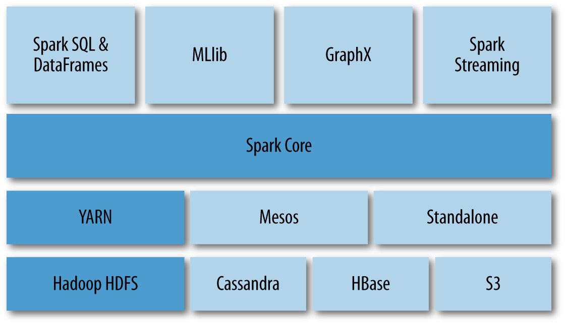
Figure 4-1. Spark is a computational framework designed to take advantage of cluster management platforms like YARN and distributed data storage like HDFS
The primary components included with Spark are as follows:
- Spark SQL
-
Originally provided APIs for interacting with Spark via the Apache Hive variant of SQL called HiveQL; in fact, you can still directly access Hive via this library. However, this library is moving toward providing a more general, structured data-processing abstraction, DataFrames. DataFrames are essentially distributed collections of data organized into columns, conceptually similar to tables in relational databases.
- Spark Streaming
-
Enables the processing and manipulation of unbounded streams of data in real time. Many streaming data libraries (such as Apache Storm) exist for handling real-time data. Spark Streaming enables programs to leverage this data similar to how you would interact with a normal RDD as data is flowing in.
- MLlib
-
A library of common machine learning algorithms implemented as Spark operations on RDDs. This library contains scalable learning algorithms (e.g., classifications, regressions, etc.). that require iterative operations across large datasets. The Mahout library, formerly the big data machine learning library of choice, will move to Spark for its implementations in the future.
- GraphX
-
A collection of algorithms and tools for manipulating graphs and performing parallel graph operations and computations. GraphX extends the RDD API to include operations for manipulating graphs, creating subgraphs, or accessing all vertices in a path.
These components combined with the Spark programming model provide a rich methodology of interacting with cluster resources. It is probably because of this completeness that Spark has become so immensely popular for distributed analytics. Instead of learning multiple tools, the basic API remains the same across components and the components themselves are easily accessed without extra installation. This richness and consistency comes from the primary programming abstraction in Spark that we’ve mentioned a few times up to this point, resilient distributed datasets, which we will explore in more detail in the next section.
Resilient Distributed Datasets
In Chapter 2, we described Hadoop as a distributed computing framework that dealt with two primary problems: how to distribute data across a cluster, and how to distribute computation. The distributed data storage problem deals with high availability of data (getting data to the place it needs to be processed) as well as recoverability and durability. Distributed computation intends to improve the performance (speed) of a computation by breaking a large computation or task into smaller, independent computations that can be run simultaneously (in parallel) and then aggregated to a final result. Because each parallel computation is run on an individual node or computer in the cluster, a distributed computing framework needs to provide consistency, correctness, and fault-tolerant guarantees for the whole computation. Spark does not deal with distributed data storage, relying on Hadoop to provide this functionality, and instead focuses on reliable distributed computation through a framework called resilient distributed datasets.
RDDs are essentially a programming abstraction that represents a read-only collection of objects that are partitioned across a set of machines. RDDs can be rebuilt from a lineage (and are therefore fault tolerant), are accessed via parallel operations, can be read from and written to distributed storages (e.g., HDFS or S3), and most importantly, can be cached in the memory of worker nodes for immediate reuse. As mentioned earlier, it is this in-memory caching feature that allows for massive speedups and provides for iterative computing required for machine learning and user-centric interactive analyses.
RDDs are operated upon with functional programming constructs that include and expand upon map and reduce. Programmers create new RDDs by loading data from an input source, or by transforming an existing collection to generate a new one. The history of applied transformations is primarily what defines the RDD’s lineage, and because the collection is immutable (not directly modifiable), transformations can be reapplied to part or all of the collection in order to recover from failure. The Spark API is therefore essentially a collection of operations that create, transform, and export RDDs.
Note
Recovering from failure in Spark is very different than in MapReduce. In MapReduce, data is written as sequence files (binary flat files containing typed key/value pairs) to disk between each interim step of processing. Processes therefore pull data between map, shuffle and sort, and reduce. If a process fails, then another process can start pulling data. In Spark, the collection is stored in memory and by keeping checkpoints or cached versions of earlier parts of an RDD, its lineage can be used to rebuild some or all of the collection.
The fundamental programming model therefore is describing how RDDs are created and modified via programmatic operations. There are two types of operations that can be applied to RDDs: transformations and actions. Transformations are operations that are applied to an existing RDD to create a new RDD—for example, applying a filter operation on an RDD to generate a smaller RDD of filtered values. Actions, however, are operations that actually return a result back to the Spark driver program—resulting in a coordination or aggregation of all partitions in an RDD. In this model, map is a transformation, because a function is passed to every object stored in the RDD and the output of that function maps to a new RDD. On the other hand, an aggregation like reduce is an action, because reduce requires the RDD to be repartitioned (according to a key) and some aggregate value like sum or mean computed and returned. Most actions in Spark are designed solely for the purpose of output—to return a single value or a small list of values, or to write data back to distributed storage.
An additional benefit of Spark is that it applies transformations “lazily”—inspecting a complete sequence of transformations and an action before executing them by submitting a job to the cluster. This lazy-execution provides significant storage and computation optimizations, as it allows Spark to build up a lineage of the data and evaluate the complete transformation chain in order to compute upon only the data needed for a result; for example, if you run the first() action on an RDD, Spark will avoid reading the entire dataset and return just the first matching line.
Programming with RDDs
Programming Spark applications is similar to other data flow frameworks previously implemented on Hadoop. Code is written in a driver program that is evaluated lazily on the driver-local machine when submitted, and upon an action, the driver code is distributed across the cluster to be executed by workers on their partitions of the RDD. Results are then sent back to the driver for aggregation or compilation. As illustrated in Figure 4-2, the driver program creates one or more RDDs by parallelizing a dataset from a Hadoop data source, applies operations to transform the RDD, then invokes some action on the transformed RDD to retrieve output.
Note
We’ve used the term parallelization a few times, and it’s worth a bit of explanation. RDDs are partitioned collections of data that allow the programmer to apply operations to the entire collection in parallel. It is the partitions that allow the parallelization, and the partitions themselves are computed boundaries in the list where data is stored on different nodes. Therefore “parallelization” is the act of partitioning a dataset and sending each part of the data to the node that will perform computations upon it.
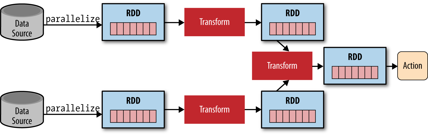
Figure 4-2. A typical Spark application parallelizes (partitions) a dataset across a cluster into RDDs
A typical data flow sequence for programming Spark is as follows:
-
Define one or more RDDs, either through accessing data stored on disk (e.g., HDFS, Cassandra, HBase, or S3), parallelizing some collection, transforming an existing RDD, or by caching. Caching is one of the fundamental procedures in Spark—storing an RDD in the memory of a node for rapid access as the computation progresses.
-
Invoke operations on the RDD by passing closures (here, a function that does not rely on external variables or data) to each element of the RDD. Spark offers many high-level operators beyond
mapandreduce. -
Use the resulting RDDs with aggregating actions (e.g.,
count,collect,save, etc.). Actions kick off the computation on the cluster because no progress can be made until the aggregation has been computed.
A quick note on variables and closures, which can be confusing in Spark. When Spark runs a closure on a worker, any variables used in the closure are copied to that node, but are maintained within the local scope of that closure. If external data is required, Spark provides two types of shared variables that can be interacted with by all workers in a restricted fashion: broadcast variables and accumulators. Broadcast variables are distributed to all workers, but are read-only and are often used as lookup tables or stopword lists. Accumulators are variables that workers can “add” to using associative operations and are typically used as counters. These data structures are similar to the MapReduce distributed cache and counters, and serve a similar role. However, because Spark allows for general interprocess communication, these data structures are perhaps used in a wider variety of applications.
Note
Closures are a cool-kid functional programming technique, and make distributed computing possible. They serve as a means for providing lexically scoped name binding, which basically means that a closure is a function that includes its own independent data environment. As a result of this independence, a closure operates with no outside information and is thus parallelizable. Closures are becoming more common in daily programming, often used as callbacks. In other languages, you may have heard them referred to as blocks or anonymous functions.
Although the following sections provide demonstrations showing how to use Spark for performing distributed computation, a full guide to the many transformations and actions available to Spark developers is beyond the scope of this book. A full list of supported transformations and actions, as well as documentation on usage, can be found in the Spark Programming Guide. In the next section, we’ll take a look at how to use Spark interactively to employ transformations and actions on the command line without having to write complete programs.
Interactive Spark Using PySpark
For datasets that fit into the memory of a cluster, Spark is fast enough to allow data scientists to interact and explore big data from an interactive shell that implements a Python REPL (read-evaluate-print loop) called pyspark. This interaction is similar to how you might interact with native Python code in the Python interpreter, writing commands on the command line and receiving output to stdout (there are also Scala and R interactive shells). This type of interactivity also allows the use of interactive notebooks, and setting up an iPython or Jupyter notebook with a Spark environment is very easy.
In this section, we’ll begin exploring how to use RDDs with pyspark, as this is the easiest way to start working with Spark. In order to run the interactive shell, you will need to locate the pyspark command, which is in the bin directory of the Spark library. Similar to how you may have a $HADOOP_HOME (an environment variable pointing to the location of the Hadoop libraries on your system), you should also have a $SPARK_HOME. Spark requires no configuration to run right off the bat, so simply downloading the Spark build for your system is enough. Replacing $SPARK_HOME with the download path (or setting your environment), you can run the interactive shell as follows:
hostname $ $SPARK_HOME/bin/pyspark
[… snip …]
>>>
PySpark automatically creates a SparkContext for you to work with, using the local Spark configuration. It is exposed to the terminal via the sc variable. Let’s create our first RDD:
>>>text = sc.textFile("shakespeare.txt")>>>print textshakespeare.txt MappedRDD[1] at textFile at NativeMethodAccessorImpl.java:-2
The textFile method loads the complete works of William Shakespeare from the local disk into an RDD named text. If you inspect the RDD, you can see that it is a MappedRDD and that the path to the file is a relative path from the current working directory (pass in a correct path to the shakespeare.txt file on your system). Similar to our MapReduce example in Chapter 2, let’s start to transform this RDD in order to compute the “Hello, World” of distributed computing and implement the word count application using Spark:
>>>from operator import add>>>def tokenize(text):...return text.split()... >>>words = text.flatMap(tokenize)
We imported the operator add, which is a named function that can be used as a closure for addition. We’ll use this function later. The first thing we have to do is split our text into words. We created a function called tokenize whose argument is some piece of text and returns a list of the tokens (words) in that text by simply splitting on whitespace. We then created a new RDD called words by transforming the text RDD through the application of the flatMap operator, and passed it the closure tokenize.
At this point, we have an RDD of type PythonRDD called words; however, you may have noticed that entering these commands has been instantaneous, although you might have expected a slight processing delay as the entirety of Shakespeare was split into words. Because Spark performs lazy evaluation, the execution of the processing (read the dataset, partition across processes, and map the tokenize function to the collection) has not occurred yet. Instead, the PythonRDD describes what needs to take place to create this RDD and in so doing, maintains a lineage of how the data got to the words form.
We can therefore continue to apply transformations to this RDD without waiting for a long, possibly erroneous or non-optimal distributed execution to take place. As described in Chapter 2, the next steps are to map each word to a key/value pair, where the key is the word and the value is a 1, and then use a reducer to sum the 1s for each key. First, let’s apply our map:
>>>wc = words.map(lambda x: (x,1))>>>print wc.toDebugString()(2) PythonRDD[3] at RDD at PythonRDD.scala:43 | shakespeare.txt MappedRDD[1] at textFile at NativeMethodAccessorImpl.java:-2 | shakespeare.txt HadoopRDD[0] at textFile at NativeMethodAccessorImpl.java:-2
Instead of using a named function, we will use an anonymous function (with the lambda keyword in Python). This line of code will map the lambda to each element of words. Therefore, each x is a word, and the word will be transformed into a tuple (word, 1) by the anonymous closure. In order to inspect the lineage so far, we can use the toDebugString method to see how our PipelinedRDD is being transformed. We can then apply the reduceByKey action to get our word counts and then write those word counts to disk:
>>>counts = wc.reduceByKey(add)>>>counts.saveAsTextFile("wc")
Once we finally invoke the action saveAsTextFile, the distributed job kicks off and you should see a lot of INFO statements as the job runs “across the cluster” (or simply as multiple processes on your local machine). If you exit the interpreter, you should see a directory called wc in your current working directory:
hostname $ ls wc/
_SUCCESS   part-00000 part-00001
Each part file represents a partition of the final RDD that was computed by various processes on your computer and saved to disk. If you use the head command on one of the part files, you should see tuples of word count pairs:
hostname $ head wc/part-00000
(u'fawn', 14)
(u'Fame.', 1)
(u'Fame,', 2)
(u'kinghenryviii@7731', 1)
(u'othello@36737', 1)
(u'loveslabourslost@51678', 1)
(u'1kinghenryiv@54228', 1)
(u'troilusandcressida@83747', 1)
(u'fleeces', 1)
(u'midsummersnightsdream@71681', 1)
Note that in a MapReduce job, the keys would be sorted due to the mandatory intermediate shuffle and sort phase between map and reduce. Spark’s repartitioning for reduction does not necessarily utilize a sort because all executors can communicate with each other and as a result, the preceding output is not sorted lexicographically. Even without the sort, however, you are guaranteed that each key appears only once across all part files because the reduceByKey operator was used to aggregate the counts RDD. If sorting is necessary, you could use the sort operator to ensure that all the keys are sorted before writing them to disk.
Writing Spark Applications
Writing Spark applications in Python is similar to working with Spark in the interactive console because the API is the same. However, instead of typing commands into an interactive shell, you need to create a complete, executable driver program to submit to the cluster. This involves a few housekeeping tasks that were automatically taken care of in pyspark—including getting access to the SparkContext, which was automatically loaded by the shell.
Many Spark programs are therefore simple Python scripts that contain some data (shared variables), define closures for transforming RDDs, and describe a step-by-step execution plan of RDD transformation and aggregation. A basic template for writing a Spark application in Python is as follows:
## Spark Application - execute with spark-submit## ImportsfrompysparkimportSparkConf,SparkContext## Shared variables and dataAPP_NAME="My Spark Application"## Closure functions## Main functionalitydefmain(sc):"""Describe RDD transformations and actions here."""passif__name__=="__main__":# Configure Sparkconf=SparkConf().setAppName(APP_NAME)conf=conf.setMaster("local[*]")sc=SparkContext(conf=conf)# Execute main functionalitymain(sc)
This template exposes the top-down structure of a Python Spark application: imports allow various Python libraries to be used for analysis as well as Spark components such as GraphX or SparkSQL. Shared data and variables are specified as module constants, including an identifying application name that is used in web UIs, for debugging, and in logging. Job-specific closures or custom operators are included with the driver program for easy debugging or to be imported in other Spark jobs, and finally some main method defines the analytical methodology that transforms and aggregates RDDs, which is run as the driver program.
Veteran Python programmers should note the use of the if __name__ == '__main__' (usually called ifmain) statement, in which the Spark configuration and SparkContext are defined and passed to the main function. The use of the ifmain allows us to easily import driver code into other Spark contexts, without creating a new context or configuration and executing a job (on import, the name won’t be __main__). In particular, Spark programmers will routinely import code from applications into an iPython/Jupyter notebook or the pyspark interactive shell to explore the analysis before running a job on a larger dataset.
The driver program defines the entirety of the Spark execution; for example, to stop or exit the program in code, programmers can use sc.stop() or sys.exit(0). This control extends to the execution environment as well—in this template, a Spark cluster configuration, local[*] is hardcoded into the SparkConf via the setMaster method. This tells Spark to run on the local machine using as many processes as available (multiprocess, but not distributed computation). While you can specify where Spark executes on the command line using spark-submit, driver programs often select this based on an environment variable using os.environ. Therefore, while developing Spark jobs (e.g., using a DEBUG variable), the job can be run locally, but in production run across the cluster on a larger data set.
Writing Spark applications is certainly different than writing MapReduce applications because of the flexibility provided by the many transformations and actions, as well as the more flexible programming environment. In the following section, we take a look at a complete analysis that leverages the centrality of the driver program to compute data across a cluster to create a visualization as output.
Visualizing Airline Delays with Spark
In Chapter 3, we explored using Hadoop Streaming and MapReduce to compute the average flight delay per airport using the US Department of Transportation’s on-time flight dataset. This kind of computation—parsing a CSV file and performing an aggregate computation—is an extremely common use case of Hadoop, particularly as CSV data is easily exported from relational databases. This dataset, which records all US domestic flight departure and arrival times along with their delays, is also interesting because while a single month is easily computed upon, the entire dataset would benefit from distributed computation due to its size.
In this example, we’ll use Spark to perform an aggregation of this dataset, in particular determining which airlines were the most delayed in April 2014. We will specifically look at the slightly more advanced (and Pythonic) techniques we can use due to the increased flexibility of the Spark Python API. Moreover, we will show how central the driver program is to the computation by pulling the results back and displaying a visualization on the driver machine using matplotlib (a task that would take two steps using traditional MapReduce).
In order to get a feel for how Spark applications are structured, and to see the template described in the previous section in action, we will first inspect a 10,000-foot view of the complete structure of the program with the details snipped out:
## Importsimportcsvimportmatplotlib.pyplotaspltfromStringIOimportStringIOfromdatetimeimportdatetimefromcollectionsimportnamedtuplefromoperatorimportadd,itemgetterfrompysparkimportSparkConf,SparkContext## Module constantsAPP_NAME="Flight Delay Analysis"DATE_FMT="%Y-%m-%d"TIME_FMT="%H%M"fields=('date','airline','flightnum','origin','dest','dep','dep_delay','arv','arv_delay','airtime','distance')Flight=namedtuple('Flight',fields)## Closure functionsdefparse(row):"""Parses a row and returns a named tuple."""passdefsplit(line):"""Operator function for splitting a line with csv module"""passdefplot(delays):"""Show a bar chart of the total delay per airline"""pass## Main functionalitydefmain(sc):"""Describe the transformations and actions used on the dataset, then plotthe visualization on the output using matplotlib."""passif__name__=="__main__":# Configure Sparkconf=SparkConf().setMaster("local[*]")conf=conf.setAppName(APP_NAME)sc=SparkContext(conf=conf)# Execute main functionalitymain(sc)
This snippet of code, while long, provides a good overview of the structure of an actual Spark program. The imports show the usual use of a mixture of standard library tools as well as a third-party library, matplotlib. As with Hadoop Streaming, any third-party code that is not part of the standard library must be either pre-installed on the cluster or shipped with the job. For code that need only be executed on the driver and not in the executors (e.g., matplotlib), you can use a try/except block and capture ImportErrors.
Note
As with Hadoop Streaming, any third-party Python dependencies that are not part of the Python standard library must be pre-installed on each node in the cluster. However, unlike Hadoop Streaming, the fact that there are two contexts, the driver context and the executor context, means that some heavyweight libraries (particularly visualization libraries) can be installed only on the driver machine, so long as they are not used in a closure passed to a Spark operation that will execute on the cluster. To prevent errors, wrap imports in a try/except block and capture ImportErrors.
The application then defines some data that is configurable, including the date and time format for parsing datetime strings and the application name. A specialized namedtuple data structure is also created in order to create lightweight and accessible parsed rows from the input data. This information should be available to all executors, but is lightweight enough to not require a broadcast variable. Next, the processing functions, parse, split, and plot are defined, as well as a main function that uses the SparkContext to define the actions and transformations on the airline dataset. Finally, the ifmain configures Spark and executes the main function.
With this high-level overview complete, let’s dive deeper into the specifics of the code, starting with the main method that defines the primary Spark operations and the analytical methodology:
## Main functionalitydefmain(sc):"""Describe the transformations and actions used on the dataset, then plotthe visualization on the output using matplotlib."""# Load the airlines lookup dictionaryairlines=dict(sc.textFile("ontime/airlines.csv").map(split).collect())# Broadcast the lookup dictionary to the clusterairline_lookup=sc.broadcast(airlines)# Read the CSV data into an RDDflights=sc.textFile("ontime/flights.csv").map(split).map(parse)# Map the total delay to the airline (joined using the broadcast value)delays=flights.map(lambdaf:(airline_lookup.value[f.airline],add(f.dep_delay,f.arv_delay)))# Reduce the total delay for the month to the airlinedelays=delays.reduceByKey(add).collect()delays=sorted(delays,key=itemgetter(1))# Provide output from the driverfordindelays:"%0.0fminutes delayed\t%s"%(d[1],d[0])# Show a bar chart of the delaysplot(delays)
Our first job is to load our two data sources from disk: first, a lookup table of airline codes to airline names, and second, the flight instances dataset. The dataset airlines.csv is a small jump table that allows us to join airline codes with the full airline name; however, because this dataset is small enough, we don’t have to perform a distributed join of two RDDs. Instead we store this information as a Python dictionary and broadcast it to every node in the cluster using sc.broadcast, which transforms the local Python dictionary into a broadcast variable.
The creation of this broadcast variable and execution is as follows. First, an RDD is created from the text file on the local disk called airlines.csv (note the relative path). Creation of the RDD is required because this data could be coming from a Hadoop data source, which would be specified with a URI to the location (e.g., hdfs:// for HDFS data or s3:// for S3, etc.). Note if this file was simply on the local machine, then loading it into an RDD is not necessary. The split function is then mapped to every element in the dataset, as discussed momentarily. Finally, the collect action is applied to the RDD, which brings the data back from the cluster to the driver as a Python list. Because the collect action was applied, when this line of code executes, a job is sent to the cluster to load the RDD, split it, then return the context to the driver program:
defsplit(line):"""Operator function for splitting a line with csv module"""reader=csv.reader(StringIO(line))returnreader.next()
The split function parses each line of text using the csv module by creating a file-like object with the line of text using StringIO, which is then passed into the csv.reader. Because there is only a single line of text, we can simply return reader.next(). While this method of CSV parsing may seem pretty heavyweight, it allows us to more easily deal with delimiters, escaping, and other nuances of CSV processing. For larger datasets, a similar methodology is applied to entire files using sc.wholeTextFiles to process many CSV files that are split into blocks of 128 MB each (e.g., the block size and replication on HDFS):
defparse(row):"""Parses a row and returns a named tuple."""row[0]=datetime.strptime(row[0],DATE_FMT).date()row[5]=datetime.strptime(row[5],TIME_FMT).time()row[6]=float(row[6])row[7]=datetime.strptime(row[7],TIME_FMT).time()row[8]=float(row[8])row[9]=float(row[9])row[10]=float(row[10])returnFlight(*row[:11])
Next, the main function loads the much larger flights.csv, which needs to be computed upon in a parallel fashion using an RDD. After splitting the CSV rows, we map the parse function to the CSV row, which converts dates and times to Python dates and times, and casts floating-point numbers appropriately. The output of this function is a namedtuple called Flight that was defined in the module constants section of the application. Named tuples are lightweight data structures that contain record information such that data can be accessed by name—for example, flight.date rather than position (e.g., flight[0]). Like normal Python tuples, they are immutable, so they are safe to use in processing applications because the data can’t be modified. Additionally, they are much more memory and processing efficient than dictionaries, and as a result, provide a noticeable benefit in big data applications like Spark where memory is at a premium.
With an RDD of Flight objects in hand, the final transformation is to map an anonymous function that transforms the RDD to a series of key/value pairs where the key is the name of the airline and the value is the sum of the arrival and departure delays. At this point, besides the creation of the airlines dictionary, no execution has been performed on the collection. However, once we begin to sum the per airline delays using the reduceByKey action and the add operator, the job is executed across the cluster, then collected back to the driver program.
At this point, the cluster computation is complete, and we proceed in a sequential fashion on the driver program. The delays are sorted by delay magnitude in the memory of the client program. Note that this is possible for the same reason that we created the airlines lookup table as a broadcast variable: the number of airlines is small and it is more efficient to sort in memory. However, if this RDD was extremely large, a distributed sort using rdd.sort could be used. Finally, instead of writing the results to disk, the output is printed to the console. If this dataset were big, the rdd.first action might be used to take the first n items rather than printing the entire dataset, or by using rdd.saveAsTextFile to write the data back to our local disk or to HDFS.
Finally, because we have the data available in the driver, we can visualize the results using matplotlib as follows:
defplot(delays):"""Show a bar chart of the total delay per airline"""airlines=[d[0]fordindelays]minutes=[d[1]fordindelays]index=list(xrange(len(airlines)))fig,axe=plt.subplots()bars=axe.barh(index,minutes)# Add the total minutes to the rightforidx,air,mininzip(index,airlines,minutes):ifmin>0:bars[idx].set_color('#d9230f')axe.annotate("%0.0fmin"%min,xy=(min+1,idx+0.5),va='center')else:bars[idx].set_color('#469408')axe.annotate("%0.0fmin"%min,xy=(10,idx+0.5),va='center')# Set the ticksticks=plt.yticks([idx+0.5foridxinindex],airlines)xt=plt.xticks()[0]plt.xticks(xt,[' ']*len(xt))# Minimize chart junkplt.grid(axis='x',color='white',linestyle='-')plt.title('Total Minutes Delayed per Airline')plt.show()
Hopefully this example illustrates the interplay of the cluster and the driver program (sending out for analytics, then bringing results back to the driver), as well as the role of Python code in a Spark application. To run this code (presuming that you have a directory called ontime with the two CSV files in the same directory), use the spark-submit command as follows:
hostname $ spark-submit app.py
Because we hardcoded the master as localhost[*] in the configuration under the ifmain, this command creates a Spark job with as many processes as are available on the localhost. It will then begin executing the transformations and actions specified in the main function with the local SparkContext. First it loads the jump table as an RDD, collect, and broadcast it to all processes, then it loads the flight data RDD and processes it to compute the average delays in a parallel fashion.
Once the context and the output from the collect is returned to the driver, we can visualize the result using matplotlib, as shown in Figure 4-4. The final result shows that the total delays (in minutes) in April 2014 span from arriving early for those you’re flying Hawaiian or Alaskan Airlines, to an aggregate total delay for most big airlines. The novelty here is not in the visualization of the analysis, but in the one-step process of submitting a parallel executing job, and in a reasonable amount of user time, displaying a result. Consequently, applications like these that deliver on-demand analyses directly to users for immediate insights are becoming increasingly common.
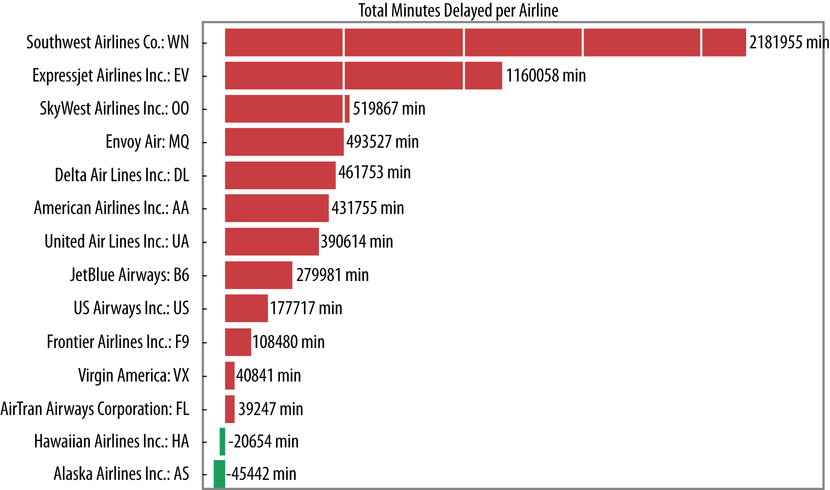
Figure 4-4. Visualization of the most delayed airlines in our dataset
Conclusion
While Spark was originally intended to address MapReduce’s limitations in performing iterative algorithms, it has now developed into a full-fledged, general-purpose distributed computation engine. Spark has evolved to cover a wide range of big data processing workloads that utilize the general-purpose engine, rather than by implementing specialized systems. Because Spark is 10–20 times faster than traditional MapReduce, you might then ask where Spark fits in the Hadoop ecosystem. While it’s premature to say that Spark is the certain successor to MapReduce, Spark is gaining an amazing amount of traction in organizations and companies that have already adopted Hadoop but are in need of a platform that can perform near real-time computations using existing cluster resources. However, we should keep in mind that at least as of now, Spark should be considered an extension of, not a replacement for, Hadoop and MapReduce, and can coexist quite well with the rest of the Hadoop ecosystem.
Spark doesn’t solve the distributed storage problem (usually Spark gets its data from HDFS), but it does provide a rich functional programming API for distributed computation. This framework is built upon the idea of resilient distributed datasets. RDDs are a programming abstraction that represents a partitioned collection of objects, allowing for distributed operations to be performed upon them. RDDs are fault tolerant (the resilient part), and most importantly, can be stored in memory on worker nodes for immediate reuse. In-memory storage provides for faster and more easily expressed iterative algorithms as well as enabling real-time interactive analyses.
Because the Spark library has an API available in Python, R, Scala, and Java, as well as built-in modules for machine learning, streaming data, graph algorithms, and SQL-like queries, it has rapidly become one of the most important distributed computation frameworks that exist today. When coupled with YARN, Spark serves to augment (not replace) existing Hadoop clusters, and will be an important part of big data in the future, opening up new avenues of data science exploration.
This chapter is far from a complete introduction to Spark; instead, it serves to introduce the Spark computing framework and resilient distributed datasets, and provide insight about how to interact with and program for Spark. Because this book is targeted toward a data science audience that knows Python or R, Spark probably feels a bit more native than Hadoop Streaming for analytics. Throughout the rest of the book, we use both Hadoop Streaming and Spark to conduct computations, but for the most part—especially where machine learning is concerned—we will primarily be using Spark.
1 Holden Karau, Andy Konwinski, Patrick Wendell, and Matei Zaharia, Learning Spark, (O’Reilly, 2015).
Get Data Analytics with Hadoop now with the O’Reilly learning platform.
O’Reilly members experience books, live events, courses curated by job role, and more from O’Reilly and nearly 200 top publishers.

